
Loading...
Loading...
Loading...
Loading...
Loading...
Loading...
Loading...
Loading...
Loading...
Loading...
Loading...
Loading...
Loading...
Loading...
Loading...
Loading...
Loading...
Loading...
Loading...
Loading...
Loading...
Loading...
Loading...
Loading...
Loading...
Loading...
Loading...
Loading...
Loading...
Loading...
Loading...
Loading...
Loading...
Loading...
Loading...
Loading...
Loading...
Loading...
Loading...
Loading...
Loading...
Loading...
Loading...
Loading...
Loading...
Loading...
Loading...
Loading...
Loading...
Loading...
Loading...
Loading...
Loading...
Loading...
Loading...
Loading...
Loading...
Loading...
Loading...
Loading...
Loading...
Loading...
Loading...
Loading...
Loading...
Loading...
Loading...
Loading...
Loading...
Loading...
Loading...
Loading...
Loading...
Loading...
Loading...
Loading...
Loading...
Loading...
Loading...
If you need support with IDC or have any questions, please open a new topic in IDC User Forum (preferred) or send email to [email protected].
Would you rather discuss your questions in an meeting with an expert from the IDC team? Book a 1-on-1 support session here: https://tinyurl.com/idc-help-request
If you are an NIH-funded investigator, you can join the that offers significant discounts on the use of cloud resources, and free training courses and materials on the use of the cloud.
If you need support with IDC or have any questions, please open a new topic in (preferred) or send email to [email protected].
Would you rather discuss your questions in an meeting with an expert from the IDC team? Book a 1-on-1 support session here:
is a cloud-based environment containing publicly available cancer imaging data co-located with analysis and exploration tools. IDC is a node within the broader NCI infrastructure that provides secure access to a large, comprehensive, and expanding collection of cancer research data.
>95 TB of data: IDC contains radiology, brightfield (H&E) and fluorescence slide microscopy images, along with image-derived data (annotations, segmentations, quantitative measurements) and accompanying clinical data
free: all of the data in IDC is publicly available: no registration, no access requests
commercial-friendly: >95% of the data in IDC is covered by the permissive CC-BY license, which allows commercial reuse (small subset of data is covered by the CC-NC license); each file in IDC is tagged with the license to make it easier for you to understand and follow the rules
cloud-based: all of the data in IDC is available from both Google and AWS public buckets: fast and free to download, no out-of-cloud egress fees
harmonized: all of the images and image-derived data in IDC is harmonized into standard DICOM representation
IDC is as much about data as it is about what you can do with the data! We maintain and actively develop a variety of tools that are designed to help you efficiently navigate, access and analyze IDC data:
exploration: start with the IDC Portal to get an idea of the data available
visualization: examine images and image-derived annotations and analysis results from the convenience of your browser using integrated OHIF, VolView and Slim open source viewers
programmatic access: use idc-index python package to perform search, download and other operations programmatically
cohort building: use rich and extensive metadata to build subsets of data programmatically using idc-index or BigQuery SQL
download: use your favorite S3 API client or idc-index to efficiently fetch any of the IDC files from our public buckets
analysis: conveniently access IDC files and metadata from the tools that are cloud-native, such as Google Colab or Looker; fetch IDC data directly into 3D Slicer using
We want Imaging Data Commons to be your companion in your cancer imaging research activities - from discovering relevant data to sharing your analysis results and showcasing the tools you developed!
Check out quick instructions on how to access and use IDC Portal web application that will help you search, subset and visualize data available in IDC.
IDC Portal is integrated with powerful visualization tools: just with your web browser you will be able to see IDC images and annotations using OHIF Viewer, Slim viewer and VolView!
We have many tools to help you search data in IDC, so that you download only what you need!
you can do basic filtering/subsetting of the data using IDC Portal, but if you are developer, you will want to learn how to use for programmatic access. will introduce you to the basics of idc-index for interaction with IDC content.
search clinical data: many of the IDC collections are accompanied by clinical data, which we parsed for you into searchable tabular representation - no need to download or parse CSV/Excel/PDF files! Dive into searching clinical data using .
if advanced content does not scare you, check out to learn how to search all of the metadata accompanying IDC using SQL and Google BigQuery.
We provide various tools for downloading data from IDC, as discussed in the . Access to all data in IDC is free! No registration. No access request forms. No logins.
once you have idc-index python package installed, download from the command line is as easy as running idc download <manifest_file>, or idc download <collection_id>.
looking for an interactive "point-and-click" application? is for you (note that you will only be able to visualize radiology - not microscopy - images in 3D Slicer)
We want to make it easier to understand performance of the latest advances in AI on real-world cancer imaging data!
if you have a Google account, you have free access to Google Colab, which allows you to run python notebooks on cloud VMs equipped with GPU - for free! Combined with idc-index for data access, this makes it rather easy to experiment with the latest AI tools! As an example, take a look at that allows you to apply MedSAM model to IDC data. You will find a growing number of notebooks to help you use IDC in .
use IDC to develop HuggingFace spaces that demonstrate the power of your models on real data: see we developed for SegVol
growing number of AI medical imaging models is being curated on the platform; see to learn how to apply those models on data from IDC
How about accompanying your next publication by a working demonstration notebook on relevant samples from IDC? You can see an example how we did this in .
With the cloud, you can do things that are simply impossible to do with your local resources.
read to learn how we applied TotalSegmentator+pyradiomics to >126,000 of CT scans of the NLST collection using Terra platform, completing the analysis in ~8 hours with the total cost ~$1000
contains the code we used in the above (this is really advanced content!)
If you have an algorithm, that you evaluated/published, that can enrich data in IDC with analysis results and you want to contribute those, or if you are a domain expert and would like to publish results of manual annotations you prepared - we want to hear from you!
IDC maintains a where we curate contributions of analysis results and other datasets produced by IDC (see the as one example of such contribution)
through a dedicated Zenodo record you will have a citation and DOI to get credit for your work; your data is ingested from Zenodo into IDC, and citation will be generated for the users of your data in IDC
once your data is in IDC, it should be easier to discover it, combine with other datasets, visualize and use from analysis workflows (as an example, see accompanying the RMS annotations)
If you need support with IDC or have any questions, please open a new topic in (preferred) or send email to [email protected].
Would you rather discuss your questions in an meeting with an expert from the IDC team? Book a 1-on-1 support session here:
Discourse (community forum):
Documentation:
GitHub organization:
Tutorials:
If you did not find the images you need in IDC, you can consider the following resources:
: while most of the public DICOM collections from TCIA are available in IDC, we do not replicate limited access TCIA collections
: list curated by Stephen Aylward
: list curated by University College London
: list curated by New York Univestity Health Sciences Library
We ingest and distribute datasets from variety of sources and contributors, primarily focusing on large data collection initiatives sponsored by US National Cancer Institute.
At this time, we do not have resources to prioritize receipt of the imaging data from individual PIs (but we are encouraging submissions of annotations/analysis results for existing IDC data!). Nevertheless, if you feel you might have a compelling dataset, please email us at [email protected].
On ingestion, we harmonize images and image-derived data into DICOM format for interoperability, whenever data is represented in a non-DICOM format.
Upon conversion, the data undergoes Extract-Transform-Load (ETL), which extracts DICOM metadata to make the data searchable, ingests the DICOM files into public S3 storage buckets and a DICOMweb store. Once the data is released, we provide various interfaces to access data and metadata.
We are actively developing a variety of capabilities to make it easier for the users to work with the data in IDC. Some of the examples of those tools include
provides interactive browser-based interface for exploration of IDC data
we are the maintainers of - an open-source viewer of DICOM digital pathology images; Slim is integrated with IDC Portal for visualizing pathology images and image-derived data available in IDC
we are actively contributing to the , and rely on it for visualizing radiology images and image-derived data
is a python package that provides convenience functions for accessing IDC data, including efficient download from IDC public S3 buckets
We welcome you to apply to contribute analysis results and annotations of the images available in IDC! These can be expert manual annotations, analysis results generated using AI tools, segmentations, contours, metadata attributes describing the data (e.g., annotation of the scan type), expert evaluation of the quality of existing AI-generated annotations in IDC.
If you would like your annotations/analysis results to be considered, you must establish the value of your contribution (e.g., describe the qualifications of the experts performing manual annotations, demonstrate robustness of the AI tool you are applying to images with a peer-reviewed publication or other type of evidence), and be willing to share your contribution under a permissive Creative Commons Attribution .
See more details on our curation policy , and reach out by sending email to with any questions or inquries. Every application will be reviewed by IDC stakeholders.
If your contribution is accepted by the IDC stakeholders:
we will work with you to choose the appropriate DICOM object type for your data and convert it into DICOM representation
upon conversion, we will create a Zenodo entry under the for your contribution so that you get the Digital Object Identifier (DOI), citation and recognition of your contribution
once published in IDC
your data will become searchable and viewable in IDC Portal, so it is easier for the users of your data to discover and work with your data
IDC is a component of the broader NCI , giving you access to the following:
can be used to find data related to the images in IDC in , and
Broad and (SB-CGC) can be used to apply analysis tools to the data in IDC (you can read more about how this can be done in from the IDC team)
platform curates a growing number of cancer imaging AI models that can be applied directly to the DICOM data available in IDC

IDC V14 introduced important enhancements to IDC data organization. The discussion of the organization of data in earlier versions is preserved here.
The following white papers are intended to provide explanation and clarification into applying DICOM to encoding specific types of data.
Comments and questions regarding those white papers are welcomed from the community! Please ask any related questions on IDC Discourse, or by adding comments directly in the documents referenced below:
Items in this section capture documentation relevant to organization of data in prior versions of IDC. Those are no longer relevant for the current data organization, and are preserved since the prior versions of data are still available to IDC users.
IDC API v1 has been released with the IDC Production release (v4).
3D Slicer extensions SlicerIDCBrowser can be used for interactive download of IDC data
we are contributing to a variety of tools that aim to simplify the use of DICOM in cancer imaging research; these include OpenSlide and BioFormats bfconvert library that can be used for conversion between DICOM Whole Slide Imaging (WSI) format and other slide microscopy formats, dcmqi library for converting image analysis results to and from DICOM representation
files can be downloaded very efficiently using S3 interface and idc-index
You can download data at the patient/case, DICOM study or series levels directly from the IDC Portal interface, as demonstrated below!
The Imaging Data Commons Portal provides a web-based interactive interface to browse the data hosted by IDC, visualize images, build manifests describing selected cohorts, and download images defined by the manifests.
The slides below give a quick guided overview of how you can use IDC Portal.
No login is required to use the portal, to visualize images, or to download data from IDC!
Imaging Data Commons team has been funded in whole or in part with Federal funds from the National Cancer Institute, National Institutes of Health, under Task Order No. HHSN26110071 under Contract No. HHSN261201500003l.
We gratefully acknowledge and the that support public hosting of IDC-curated content, and cover out-of-cloud egress fees!
Several of the members of the IDC team utilize compute resources supported via the
IDC Portal offers lots of flexibility in selecting items to download. In all cases, download of data from IDC Portal is a two step process:
Select items and export a manifest corresponding to your selection.
Use command-line python tool or 3D Slicer IDC browser extension to download the files for your selection, as discussed in .
IDC supports a variety of interfaces for fetching individual images, cohorts (groups of images), or portions of images, using desktop application, command-line interface, or programmatic API. These interfaces are covered in the subsequent pages. You should select the specific approach to accessing IDC data depending on your requirements.
Download directly from : no prerequisites other than a Chrome web browser!
DICOM defines its own model to map relevant entities from the real world. That model, as , is shown in the figure below.
The DICOM data model is implicit, and is not defined in a machine-readable structured form by the standard!
DICOM data model entities do not always map to DICOM objects! In fact, every DICOM object you will ever encounter in IDC will contain attributes describing various properties of the entries at different levels of the real world data model. Such objects are called Composite Information Objects. The of the Composite Information Object Definitions is shown below, and covers all of the composite objects defined by the standard.
DICOM and TIFF are two different image file formats that share many similar characteristics, and are capable of encoding exactly the same pixel data, whether uncompressed, or compressed with common lossy schemes (including JPEG and JPEG 2000). This allow the pixel data to be losslessly transformed from one format to the other and back.
The DICOM file format was also deliberately designed to allow the two formats (TIFF and DICOM) to peacefully co-exist in the same file, sharing the same pixel data without expanding the file size significantly. This is achieved by leaving some unused space at the front of the DICOM file ("preamble"), which allows for the presence of a TIFF format recognition code ("magic number") and a pointer to its Image File Directory (IFD), which in turn contains pointers into the shared DICOM Pixel Data element.
The dual-personality mechanism supports both traditional strip-based TIFF organization, such as might be used to encode a single frame image, as well as the tile-based format, which is commonly used for Whole Slide Images (WSI), and which is encoded in DICOM with each tile as a frame of a "multi-frame" image.
Unlike TIFF files, which allow multiple different sized images to be encoded in the same file, DICOM does not, so there are limits to this approach. For example, though an entire WSI pyramid can be encoded in a TIFF file, the DICOM WSI definition requires each pyramid layer to be in a separate file, and all frames (tiles) within the same file to be the same size.
Most of the structural metadata that describes the organization and encoding of the pixel data is similar in DICOM and TIFF. It is copied into the tags (data elements) encoded in the respective format "headers". Biomedical-specific information, such as patient, specimen and anatomical identifiers and descriptions, as well as acquisition technique, is generally only encoded in the DICOM data elements, their being no corresponding standard TIFF tags for it. Limited spatial information (such as physical pixel size) can be encoded in TIFF tags, but more complex multi-dimensional spatial location is standardized only in the DICOM data elements.
Topic-specific dashboards
The primary mechanism for accessing data from IDC is by searching the metadata using the idc-index python package or BigQuery tables, and downloading the binary files from public cloud buckets, as discussed in . There is no limit, quota or fees associated with downloading IDC files from the buckets.
Effective March 2024, as a pilot project, IDC also provides access to the DICOM data via the DICOMweb interface available at this endpoint: . This endpoint is read-only. It will route the requests to the Google Healthcare API DICOM store containing IDC data.
Our DICOMWeb endpoint should only be used when data access needs cannot be satisfied using other mechanisms (e.g., when accessing individual frames of the microscopy images without having to download the entire binary file).
Egress of data via the DICOMweb interface is capped at a non-disclosed limit that is tracked per IP. It is not acceptable to “IP hop” in an attempt to circumvent individual daily quotas, since there is also a global daily cap as well to prevent full egress of the imaging collection. Note that if this global cap is hit, all other users of the site would be unable to use the viewers for the rest of the day (using the UTC clock). Thus, IP hopping against the proxy that causes the global quota to be hit will be considered a denial-of-service attack.
As of 15-July-2025, support for user defined cohorts has been removed from the both the IDC API V1 and the IDC API V2. The API documentation has been revised accordingly.
This section describes version 2 of the IDC REST API . The documentation for the version 1 API will be found .
This API is designed for use by developers of image analysis and data mining tools to directly query the public resources of the IDC and retrieve information into their applications. The API complements the IDC web application but eliminates the need for users to visit the IDC web pages to perform manifest export, and transfer of image data to some local file system.
The IDC API conforms to the specification which "defines a standard, language-agnostic interface to RESTful APIs which allows both humans and computers to discover and understand the capabilities of the service without access to source code, documentation, or through network traffic inspection."
Note: As of 15-July-2025, support for user defined cohorts has been removed from the both the IDC API V1 and the IDC API V2. The API documentation has been revised accordingly.
This section describes v1 of the IDC REST API . This API is designed for use by developers of image analysis and data mining tools to directly query the public resources of the IDC and retrieve information into their applications. The API complements the IDC web application but eliminates the need for users to visit the IDC web pages to perform cohort creation, manifest export, and transfer of image data to some local file system.
The IDC API conforms to the specification which "defines a standard, language-agnostic interface to RESTful APIs which allows both humans and computers to discover and understand the capabilities of the service without access to source code, documentation, or through network traffic inspection."
This section of the documentation complements the tutorials available in our notebooks repository:
: all of the pathology images in IDC are in DICOM Slide Microscopy format; this notebook will help you get started with using this representation and also searching IDC pathology images.
: introduction to the key metadata accompanying IDC slide microscopy images that can be used for subsetting data and building cohorts.
In the following subsections you will find notebooks that don't require python programming, or have dependencies that make them not suitable for the python notebook format.
Search results are updated dynamically based on the search configuration. At any time you can expand the items on the right to explore the selected collections, cases, studies and series.
Studies and series tables include the button to open those in the browser-based image viewer.
See IDC API endpoint details at .
is a free tool that turns your data into informative, easy to read, easy to share, and fully customizable dashboards and reports.
In this section you can learn how to very quickly make a custom Looker Studio dashboard to explore the content of your cohort, and find some additional examples of using Looker Studio for analyzing content of IDC.
are components of the that bring data and computational power together to enable cancer research and discovery.
Our current experience in using NCI Cloud Resources for cancer image analysis is summarized in the following preprint:
Thiriveedhi, V. K., Krishnaswamy, D., Clunie, D., Pieper, S., Kikinis, R. & Fedorov, A. Cloud-based large-scale curation of medical imaging data using AI segmentation. Research Square (2024). doi:
Since IDC data is available via standard interfaces, you can use any of the tool supporting those interfaces to access the data. This page provides pointers to some of such tools that you might find useful.
If you are aware of any other tool that is not listed here, but is helpful for accessing IDC data, please let us know on the , and we will be happy to add it here!
: open-source Python interface to ,
This section contains various recipes that might be useful in utilizing GCP Compute Engine (GCE).
You are also encouraged to review the slides in the following presentation that provides an introduction into GCE, and shares some best practices the its usage.
W. Longabaugh. Introduction to Google Cloud Platform. Presented at MICCAI 2021. ()
The dictionary of TIFF tags can be extended with application-specific entries. This has been done for various non-medical and medical applications (e.g., GeoTIFF, DNG, DEFF). Other tools have used alternative mechanisms, such as defining text string (Leica/Aperio SVS) or structured metadata in other formats (such as XML for OME) buried within a TIFF string tag (e.g, ImageDescription). This approach can be used with DICOM-TIFF dual-personality files as well, since DICOM does not restrict the content of the TIFF tags; it does require updating or crafting of the textual metadata to actually reflect the characteristics of the encoded pixel data.
It is hoped that the dual-personality approach may serve to mitigate the impact of limited support of one format or the other in different clinical and research tools for acquisition, analysis, storage, indexing, distribution, viewing and annotation.
idc-index interface: command-line and Python API interface to download images corresponding to the specific patient/study/series, or a cohort defined by a manifest
3D Slicer interface: desktop application to download images corresponding to the specific patient/study/series, or a cohort defined by a manifest
s5cmd: command-line interface to download images for a cohort defined by a manifest (unlike idc-index, does not organize downloaded images into folders corresponding to IDC data model hierarchy)
DICOMweb interface: REST API interface to access both metadata and pixel data at the granularity of image frames/tiles
Directly loading DICOM objects from Google Cloud or AWS in Python: Python API interface to access both metadata and pixel data at the granularity of image frames/tiles
Program- and Collection-specific dashboards
LIDC-IDRI collection dashboard (see details in this paper)
If you reach your daily quota, but feel you have a compelling cancer imaging research use case to request an exception to the policy and an increase in your daily quota, please reach out to us at [email protected] to discuss the situation.
We are continuously monitoring the usage of the proxy. Depending on the actual costs and usage, this policy may be revisited in the future to restrict access via the DICOMweb interface for any uses other than IDC viewers.
If you have feedback about the desired features of the IDC API, please let us know via the IDC support forum.
The API is a RESTful interface, accessed through web URLs. There is no software that an application developer needs to download in order to use the API. The application developer can build their own access routines using just the API documentation provided. The interface employs a set of predefined query functions that access IDC data sources.
The IDC API is intended to enable exploration of IDC hosted data without the need to understand and use the Structure Query Language (SQL). To this end, data exploration capabilities through the IDC API are limited. However, IDC data is hosted using the standard capabilities of the the Google Cloud Platform (GCP) Storage (GCS) and BigQuery (BQ) components. Therefore, all of the capabilities provided by GCP to access GCS storage buckets and BQ tables are available for more advanced interaction with that data.
SwaggerUI is a web based interface that allows users to try out APIs and easily view their documentation. You can access the IDC API SwaggerUI here.
This Google Colab notebook serves as an interactive tutorial to accessing the IDC API using Python.
You will see "Cart" icon in the search results collections/cases/studies/series tables. Any of the items in these tables can be added to the cart for subsequent downloading of the corresponding files.
Get the manifest for the cart content using "Manifest" button in the Cart panel.
Clicking "Manifest" button in the "Cohort Filters" panel will given you the manifest for all of the studies that match your current selection criteria.
Studies table contains a button for downloading manifest that will contain references to the files in the given study. To download a single series, no manifest is needed. You will see the command line to run to do the download.
If you would like to download the entire study, or the specific image you see in the image viewer, you can use the download button in the viewer interface.
As can be observed from this diagram, "each Composite Instance IOD [Entity-Relationship] Model requires that all Composite Instances that are part of a specific Study shall share the same context. That is, all Composite Instances within a specific Patient Study share the same Patient and Study information; all Composite Instances within the same Series share the same Series information; etc." (ref).
Each of the boxes in the diagram above corresponds to Information Entities (IEs), which in turn are composed from Information Modules. Information Modules group attributes that are related. As an example, Patient IE included in the MR object will include Patient Information Module, which in turn will include such attributes as PatientID, PatientName, and PatientSex.
Click on the "i" button to toggle information panel about the individual items in the search panels
Cohort filters panel: get the shareable URL for the current selection by clicking "URL" button in the Cohort Filters panel
Get the manifest for downloading all of the matching studies by clicking "Manifest" button in the Cohort Filters panel

You can copy identifiers of the individual collections, cases, studies or series to the clipboard - those can be used to download corresponding files as discussed in the Downloading data section - using command-line download tool or 3D Slicer IDC extension
IDC and TCIA are partners in providing FAIR data for cancer imaging researchers.
TCIA provides unique service to work with data submitters to de-identify cancer imaging data and make it available for download.
The mission of IDC is to support efficient access and use of the cancer imaging data, after it was de-identified and released.
Here are some of the highlights that make IDC unique:
Unique datasets: while all of the public TCIA DICOM collections are available in IDC, there is a growing amount of data in IDC that is not available anywhere else:
DICOM digital pathology collections from prominent initiatives: Childhood Cancer Data Initiative (CCDI), GTEx, TCGA, CPTAC, HTAN, CMB
image analysis results available only from IDC, such as TotalSegmentator segmentations and radiomics features for most of the CT images in the NLST collection
Cloud-native: IDC makes the data available in public cloud buckets, the egress is free (TCIA provides download from on-premises servers at a single institution): chances are your will be able to download data from IDC much faster than from TCIA
Partnerships with cloud vendors: IDC collaborates with Public Datasets Programs of Amazon Web Services and Google Cloud to support hosting and free out-of-cloud egress, contributing to improved accessibility, sustainability and longevity of the resource
State of the art tools: IDC maintains superior community recognized tools to support the use of the data:
modern OHIF Viewer v3 for radiology data, with support of visualization of annotations and segmentations;
Slim viewer for digital pathology and annotations
highly capable IDC Portal
Standard access interfaces: IDC offers standard interfaces for data access: S3 API for file download, DICOMweb for interoperability with DICOM tools, SQL for searching all of the DICOM metadata (TCIA offers various non-standard, in-house interfaces and APIs for data access)
Harmonized data: All of the data (radiology and digital pathology images, annotations, segmentations, image-derived features) available in IDC is harmonized into DICOM representation, which means
interoperability: you can use IDC data with any DICOM-compatible tool
metadata: every single file in IDC is accompanied by metadata that follows DICOM data model, and is associated with unique identifiers, allowing you to build reproducible cohorts
uniform representation: you don't need to customize your processing pipelines to a specific collection, and can build cohorts combining data across collections
Co-location with cloud compute resources: IDC data is easier to access from cloud computing resources, allowing you to more easily experiment with the new analysis tools and scale your computation
Versioning: IDC data is versioned: you will be able to access the exact files you analyzed in a given verison of IDC even if there were any updates to the collection after you accessed it, helping you achieve reproducibility of your analyses
Open-source tool stack: all of the tools developed by IDC are shared under permissive licenses to support community contribution, reuse and sustainability
Check out the documentation page!
Note that currently IDC prioritizes submissions from NCI-funded driving projects and data from special selected projects.
If you would like to submit images, it will be your responsibility to de-identify them first, documenting the de-identification process and submitting that documentation for the review by IDC stakeholders.
We welcome submissions of image-derived data (expert annotations, AI-generated segmentations) for the images already in IDC, see IDC Zenodo community to learn about the requirements for such submissions!
IDC works closely with and mirrors TCIA public collections. If you submit your DICOM data to TCIA and your data is released as a public collection, it will be automatically available in IDC in a following release.
If you are interested in making your data available within IDC, please contact us by sending email to .
IDC data is stored in the cloud buckets, and you can search and for free and without login.
If you would like to use the cloud for analysis of the data, we recommend you start with the free tier of to get free access to a cloud-hosted VM with GPU to experiment with analysis workflows for IDC data. If you are an NIH-funded researcher, you may be eligible for a free allocation via . US-based researchers can also access free cloud-based computing resources via .
IDC pilot release took place in Fall 2020, followed by the production release in September 2021. IDC team is continuously refining the capabilities of IDC Portal and various tools, and publishes new data releases every 3-4 months.
We host most of the public collections from . We also host HTAN and other pathology images not hosted by TCIA. You can review the complete, up-to-date list of .
Please cite the latest paper from the IDC team. Please also make sure you acknowledge the specific data collections you used in your analysis.
Fedorov, A., Longabaugh, W. J. R., Pot, D., Clunie, D. A., Pieper, S. D., Gibbs, D. L., Bridge, C., Herrmann, M. D., Homeyer, A., Lewis, R., Aerts, H. J. W. L., Krishnaswamy, D., Thiriveedhi, V. K., Ciausu, C., Schacherer, D. P., Bontempi, D., Pihl, T., Wagner, U., Farahani, K., Kim, E. & Kikinis, R. National cancer institute imaging data commons: Toward transparency, reproducibility, and scalability in imaging artificial intelligence. Radiographics 43, (2023).
The main website for the Cancer Research Data Commons (CRDC) is
Clinical data that was shared by the submitters is available for a number of imaging collections in IDC. Please see on how to search that data and how to link clinical data with imaging metadata!
Many of the imaging collections are also accompanied by the genomics or proteomics data. CRDC provides the API to locate such related datasets.
IDC Portal gives you access to just a small subset of the metadata accompanying IDC images. If you want to learn more about what is available, you have several options:
from our Getting Started tutorial series explains how to use - a python package that aims to simplify access to IDC data
will help you get started with searching IDC metadata in BigQuery, which gives you access to all of the DICOM metadata extracted from IDC-hosted files
if you are not comfortable writing queries or coding in pyhon, you can use to search using some of the attributes that are not available through the portal. You can also to include additional attributes.
IDC relies on DICOM data model for organizing images and image-derived data. At the same time, IDC includes certain attributes and data types that are outside of the DICOM data model. The Entity-Relationship (E-R) diagram and examples below summarize a simplified view of the IDC data model (you will find the explanation of how to interpret the notation used in this E-R diagram in this page from Mermaid documentation).
IDC content is organized in Collections: groups of DICOM files that were collected through certain research activity.
Collections are organized into Programs, which group related collections, or those collections that were contributed under the same funding initiative or a consortium. Example: TCGA program contains TCGA-GBM, TCGA-BRCA and other collections. You will see Collections nested under Programs in the upper left section of the IDC Portal. You will also see the list of collections that meet the filter criteria in the top table on the right-hand side of the portal interface.
Individual DICOM files included in the collection contain attributes that organize content according to the DICOM data model.
Each collection will contain data for one or more case, or patient. Data for the individual patient is organized in DICOM studies, which group images corresponding to a single imaging exam/enconter, and collected in a given session. Studies are composed of DICOM series, which in turn consist of DICOM instances. Each DICOM instance correspond to a single file on disk. As an example, in radiology imaging, individual instances would correspond to image slices in multi-slice acquisitions, and in digital pathology you will see a separate file/instance for each resolution layer of the image pyramid. When using IDC Portal, you will never encounter individual instances - you will only see them if you download data to your computer.
Analysis results collection is a very important concept in IDC. These contain analysis results that were not contributed as part of any specific collection. Such analysis results might be contributed by investigators unrelated to those that submitted the analyzed images, and may span images across multiple collections.
One of the fundamental principles of DICOM is the use of controlled terminologies, or lexicons, or coding schemes (for the purposes of this guide, these can be used interchangeably). While using the DICOM data stored in IDC, you will encounter various situations where the data is captured using coded terms.
Controlled terminologies define a set of codes, and sometimes their relationships, that are carefully curated to describe entities for a certain application domain. Consistent use of such terminologies helps with uniform data collection and is critical for harmonization of activities conducted by independent groups.
When codes are used in DICOM, they are saved as triplets that consist of
CodeValue: unique identifier for a term
CodingSchemeDesignator: code for the authority that issued this code
CodeMeaning: human-readable code description
DICOM relies on various sources of codes, all of which are listed in of the standard.
As an example, if you query the view with the following query in the BQ console:
You will see columns that contain coded attributes of the segment. In the example below, the value of AnatomicRegion corresponding to the segment is assigned the value (T-04000, SRT, Breast), where "SRT" is the coding scheme designator corresponding to the coding scheme.
As another example, quantitative and qualitative measurements extracted from the SR-TID1500 objects are stored in the and views, respectively. If we query those views to see the individual measurements, they also show up as coded items. Each of the quantitative measurements includes a code describing the quantity being measured, the actual numeric value, and a code describing the units of measurement:
DICOM SR uses data elements to encode a higher level abstraction that is a tree of content, where nodes of the tree and their relationships are formalized. SR-TID1500 is one of many standard templates that define constraints on the structure of the tree, and is intended for generic tasks involving image-based measurements. DICOM SR uses standard terminologies and codes to deliver structured content. These codes are used for defining both the concept names and values assigned to those concepts (name-value pairs). Measurements include coded concepts corresponding to the quantity being measured, and a numeric value accompanied by coded units. Coded categorical or qualitative values may also be present. In SR-TID1500, measurements are accompanied by additional context that helps interpret and reuse that measurement, such as finding type, location, method and derivation. Measurements computed from segmentations can reference the segmentation defining the region and the image segmented, using unique identifiers of the respective objects.
At this time, only the measurements that accompany regions of interest defined by segmentations are exposed in the IDC Portal, and in the measurements views maintained by IDC!
Open source DCMTK tool can be used to render the content of the DICOM SR tree in a human-readable form (you can see one example of such rendering ). Reconstructing this content using tools that operate with DICOM content at the level of individual attributes can be tedious. We recommend the tools referenced above that also provide capabilities for reading and writing SR-TID1500 content:
: high-level DICOM abstractions for the Python programming language
: open source DCMTK-based C++ library and command line converters that aim to help with the conversion between imaging research formats and the standard DICOM representation for image analysis results
: C++ library that provides API abstractions for reading and writing SR-TID1500 documents
Tools referenced above can be used to 1) extract qualitative evaluations and quantitative measurements fro the SR-TID1500 document; 2) generate standard-compliant SR-TID1500 objects.
We differentiate between the original and derived DICOM objects in the IDC portal and discussions of the IDC-hosted data. By Original objects we mean DICOM objects that are produced by image acquisition equipment - MR, CT, or PET images fall into this category. By Derived objects we mean those objects that were generated by means of analysis or annotation of the original objects. Those objects can contain, for example, volumetric segmentations of the structures in the original images, or quantitative measurements of the objects in the image.
Most of the images stored on IDC are saved as objects that store individual slices of the image in separate instances of a series, with the image stored in the PixelData attribute.
As of production release, IDC contains both radiology and digital pathology images. The following publication can serve as a good introduction into the use of DICOM for digital pathology.
Herrmann, M. D., Clunie, D. A., Fedorov, A., Doyle, S. W., Pieper, S., Klepeis, V., Le, L. P., Mutter, G. L., Milstone, D. S., Schultz, T. J., Kikinis, R., Kotecha, G. K., Hwang, D. H., Andriole, K. P., John Lafrate, A., Brink, J. A., Boland, G. W., Dreyer, K. J., Michalski, M., Golden, J. A., Louis, D. N. & Lennerz, J. K. Implementing the DICOM standard for digital pathology. J. Pathol. Inform. 9, 37 (2018).
Open source libraries such as DCMTK, GDCM, ITK, and pydicom can be used to parse such files and load pixel data of the individual slices. Recovering geometry of the individual slices (spatial location and resolution) and reconstruction of the individual slices into a volume requires some extra consideration.
: command-line tool to convert neuroimaging data from the DICOM format to the NIfTI format
: open source software for image computation, which includes
: python library providing API and command-line tools for converting DICOM images into NIfTI format
Indexing of the collection of NSCLC-Radiomics by the Data Commons Framework is pending.
QIN multi-site collection of Lung CT data with Nodule Segmentations: only items corresponding to the LIDC-IDRI original collection are included
DICOM SR of clinical data and measurement for breast cancer collections to TCIA: only items corresponding to the ISPY1 original collection are included
: Some of the segmentations in this collection are empty (as an example, SeriesNumber 42100 with SeriesDescription "VOI PE Segmentation thresh=70" in is empty).
Due to the existing limitations of Google Healthcare API, not all of the DICOM attributes are extracted and are available in BigQuery tables. Specifically:
sequences that have more than 15 levels of nesting are not extracted (see ) - we believe this limitation does not affect the data stored in IDC
sequences that contain around 1MiB of data are dropped from BigQuery export and RetrieveMetadata output currently. 1MiB is not an exact limit, but it can be used as a rough estimate of whether or not the API will drop the tag (this limitation was not documented as of writing this) - we know that some of the instances in IDC will be affected by this limitation. The fix for this limitation is targeted for sometime in 2021, according to the communication with Google Healthcare support.
IDC provides a variety of interfaces to access both the data (as files) and metadata (to subset files and build cohorts). The flow of data and the relationship between the various components IDC uses is summarized in the following figure.
We maintain the following resources to enable access to IDC data:
Cloud storage buckets: files maintained by IDC are mirrored between Google and AWS public storage buckets that provide fee-free egress without requiring login. The buckets organize files by DICOM series, each series stored in a separate folder. Given the large overall size of data in IDC, you will likely need to use one of the search interfaces to identify relevant series first.
BigQuery tables: collection-level metadata, DICOM metadata, clinical data tables available via SQL query interface.
Python API: pip-installable provides programmatic interface and command-line tools to search IDC data using most important metadata attributes, and to download files corresponding to the selected cohorts from the cloud buckets
: alternative language-independent API for selecting subsets of data
: DICOM files and metadata queries available from Google Healthcare DICOM stores
DICOM Radiotherapy Structure Sets (RTSS, or RTSTRUCT) define regions of interest by a set of planar contours.
RTSS objects can be identified by the RTSTRUCT value assigned to the Modality attribute, or by SOPClassUID = 1.2.840.10008.5.1.4.1.1.481.3.
If you use the IDC Portal, you can select cases that include RTSTRUCT objects by selecting "Radiotherapy Structure Set" in the "Original" tab, "Modality" section (filter link). Here is a sample study that contains an RTSS series.
As always, you get most of the power in exploring IDC metadata when using SQL interface. As an example, the query below will select a random study that contains a RTSTRUCT series, and return a URL to open that study in the viewer:
# get the viewer URL for a random study that
# contains RTSTRUCT modality
SELECT
ANY_VALUE(CONCAT("https://viewer.imaging.datacommons.cancer.gov/viewer/", StudyInstanceUID)) as viewer_url
FROM
`bigquery-public-data.idc_current.dicom_all`
WHERE
StudyInstanceUID IN (
# select a random DICOM study that includes an RTSTRUCT object
SELECT
StudyInstanceUID
FROM
`bigquery-public-data.idc_current.dicom_all`
WHERE
SOPClassUID = "1.2.840.10008.5.1.4.1.1.481.3"
ORDER BY
RAND()
LIMIT
1)RTSTRUCT relies on unstructured text in describing the semantics of the individual regions segmented. This information is stored in the StructureSetROISequence.ROIName attribute. The following query will return the list of all distinct values of ROIName and their frequency.
We recommend tool for converting planar contours of the individual structure sets into volumetric representation.
The following characteristics apply to all IDC APIs:
You access a resource by sending an HTTP request to the IDC API server. The server replies with a response that either contains the data you requested, or a status indicator.
An API request URL has the following structure: <BaseURL><API version><QueryEndpoint>?<QueryParameters>. For example, this curl command is a request for metadata on all IDC collections:
curl -X GET "https://api.imaging.datacommons.cancer.gov/v1/collections" -H "accept: application/json"
Authorization
Some of the APIs, such as /collections and /cohorts/preview, can be accessed without authorization. APIs that access user specific data, such as cohorts, necessarily require account authorization.
To access these APIs that require IDC authorization, you will need to generate a credentials file. To obtain your credentials:
Clone the to your local machine.
Execute the idc_auth.py script either through the command line or from within python. Refer to the idc_auth.py file for detailed instructions.
Example usage of the generated authorization is demonstrated by code in the Google Colab notebook.
Several IDC APIs, specifically /cohorts/manifest/preview, /cohorts/manifest/{cohort_id}, /cohorts/query/preview, /cohorts/query/{cohort_id}, and /dicomMetadata, are paged. That is, several calls of the API may be required to return all the data resulting from such a query. Each accepts a _page_size query parameter that is the maximum number of objects that the client wants the server to return. The returned data from each of these APIs includes a next_page value. next_page is null if there is no more data to be returned. If next_page is non-null, then more data is available.
There are corresponding queries, /cohorts/manifest/nextPage, /cohorts/query/nextPage, and /dicomMetadata/nextpage endpoints, that each accept two query parameters: next_page, and page_size. In the case that the returned next_page value is not null, the corresponding ../nextPage endpoint is accessed, passing the next_page token returned by the previous call.
The manifest and query endpoints may return an HTTP 202 error. This indicates that the request was accepted but processing timed out before it was completed. In this case the client should resubmit the request including the next_page token that was returned with the error response.
This page provides details on each of the IDC API endpoints.
The Imaging Data Commons Portal provides a web-based interactive interface to browse the data hosted by IDC, visualize images, build manifests describing selected cohorts, and download images defined by the manifests.
The slides below give a quick guided overview of how you can use IDC Portal.
No login is required to use the portal, to visualize images, or to download data from IDC!
Components on the left side of the page give you controls for configuring your selection:
Search scope allows you to limit your search to just the specific programs, collections and analysis results (as discussed in the documentation of the IDC Data model).
Search configuration gives you access to a small set of metadata attributes to select DICOM studies (where "DICOM studies" fit into IDC data model is also discussed in the page) that contain data that meets the search criteria.
Panels on the right side will automatically update based on what you select on the left side!
Selection configuration reflects the active search scope/filters in the Cohort Filters section. You can download all of the studies that match your filters. Below you will see the Cart section. Cart is helpful when selecting data by individual filters is too imprecise, and you want to have more granular control over your selection by selecting specific collections/patients/studies/series.
Filtering results section consists of the tables containing matching content that you can navigate following IDC Data model: first table shows the matching collections, selecting a collection will list matching cases (patients), selection of a case will populate the next table listing matching studies for the patient, and finally selecting a study will expand the final table with the list of series included in the study.
In the following sections of the documentation you will learn more about each of the items we just discussed.
Most of the data in IDC is received from the data collection initiatives/projects supported by US National Cancer Institute. Whenever source images or image-derived data is not in the DICOM format, it is harmonized into DICOM as part of the ingestion.
As of data release v21, IDC sources of data include:
DICOM Segmentation object (SEG) can be identified by SOPClassUID= 1.2.840.10008.5.1.4.1.1.66.4 Unlike most "original" image objects that you will find in IDC, SEG belongs to the family of enhanced multiframe image objects, which means that it stores all of the frames (slices) in a single object. SEG can contain multiple segments, a segment being a separate label/entity being segmented, with each segment containing one or more frames (slices). All of the frames for all of the segments are stored in the PixelData attribute of the object.
If you use the IDC Portal, you can select cases that include SEG objects by selecting "Segmentations" in the "Modality" section () under the "Original" tab . Here is that contains a SEG series.
You can further explore segmentations available in IDC via the "Derived" tab of the Portal by filtering those by specific types and anatomic locations. As an example, will select cases that contain segmentations of a nodule.
In this section we discuss derived DICOM objects, including annotations, that are stored in IDC. It is important to recognize that, in practice, annotations are often shared in non-standard formats. When IDC ingests a dataset where annotations are available in such a non-standard representation, those need to be harmonized into a suitable DICOM object to be available in IDC. Due to the complexity of this task, we are unable to perform such harmonization for all of the datasets. If you want to check if there are annotations in non-DICOM format available for a given collection, you should locate the original source of the data, and examine the accompanying documentation for available non-DICOM annotations.
As an example, the collection is available in IDC. If you mouse over the name of that collection in the IDC Portal, the tooltip will provide the overview of the collection and the link to the source.
SELECT
structureSetROISequence.ROIName AS ROIName,
COUNT(DISTINCT(SeriesInstanceUID)) AS ROISeriesCount
FROM
`bigquery-public-data.idc_current.dicom_all`
CROSS JOIN
UNNEST (StructureSetROISequence) AS structureSetROISequence
WHERE
SOPClassUID = "1.2.840.10008.5.1.4.1.1.481.3"
GROUP BY
ROIName
ORDER BY
ROISeriesCount DESCMetadata describing the segments is contained in the SegmentSequence of the DICOM object, and is also available in the BigQuery table view maintained by IDC in the bigquery-public-data.idc_current.segmentations BigQuery table. That table contains one row per segment, and for each segment includes metadata such as algorithm type and structure segmented.
We recommend you use one of the following tools to interpret the content of the DICOM SEG and convert it into alternative representations:
dcmqi: open source DCMTK-based C++ library and command line converters that aim to help with the conversion between imaging research formats and the standard DICOM representation for image analysis results
highdicom: high-level DICOM abstractions for the Python programming language
DCMTK: C++ library that provides API abstractions for reading and writing SEG objects
Tools referenced above can be used to 1) extract volumetrically reconstructed mask images corresponding to the individual segments stored in DICOM SEG; 2) extract segment-specific metadata describing its content; 3) generate standard-compliant DICOM SEG objects from research formats.
# get the viewer URL for a random study that
# contains SEG modality
SELECT
ANY_VALUE(CONCAT("https://viewer.imaging.datacommons.cancer.gov/viewer/", StudyInstanceUID)) as viewer_url
FROM
`bigquery-public-data.idc_current.dicom_all`
WHERE
StudyInstanceUID IN (
# select a random DICOM study that includes a SEG object
SELECT
StudyInstanceUID
FROM
`bigquery-public-data.idc_current.dicom_all`
WHERE
SOPClassUID = "1.2.840.10008.5.1.4.1.1.66.4"
ORDER BY
RAND()
LIMIT
1)all DICOM files from the public collections are mirrored in IDC
a subset of digital pathology collections and analysis results harmonized from vendor-specific representation (as available from TCIA) into DICOM Slide Microscopy (SM) format
Childhood Cancer Data Initiative (CCDI) (ongoing)
digital pathology slides harmonized into DICOM SM
The Cancer Genome Atlas (TCGA) slides harmonized into DICOM SM
Human Tumor Atlas Network (HTAN)
release 1 of the HTAN data harmonized into DICOM SM
National Library of Medicine Visible Human Project
v1 of the Visible Human images harmonized into DICOM MR/CT/XC
Genotype-Tissue Expression Project (GTex)
digital pathology slides harmonized into DICOM SM
The list of all of the IDC collections is available in IDC Portal here: https://portal.imaging.datacommons.cancer.gov/collections/.
Whenever IDC replicates data from a publicly available source, we include the reference to the origin:
from the IDC Portal Explore page, click on the "i" icon next to the collection in the collections list
source_doi metadata column contains Digital Object Identifier (DOI) at the granularity of the individual files and is available both via python idc-index package (see this tutorial on how to access it) and BigQuery interfaces
Check out Data release notes for information about the collections added in the individual IDC data releases.
Simplified workflow for IDC data ingestion is summarized in the following diagram.
You will also find the link to the source in the list of collections available in IDC.
Finally, if you select data using SQL, you can use the source_DOI and/or the source_URL column to identify the source of each file in the subset you selected (learn more about source_DOI, licenses and attribution in the part 3 of our Getting started tutorial).
For the collection in question, the source DOI is https://doi.org/10.7937/e4wt-cd02, and on examining that page you will see a pointer to the CSV file with the coordinates of the bounding boxes defining regions containing lesions.
Non-standard annotations are not searchable, usually are not possible to visualize in off-the-shelf tools, and require custom code to interpret and parse. The situation is different for the DICOM derived objects that we discuss in the following sections.
In IDC we define "derived" DICOM objects as those that are obtained by analyzing or post-processing the "original" image objects. Examples of derived objects can be annotations of the images to define image regions, or to describe findings about those regions, or voxel-wise parametric maps calculated for the original images.
Although DICOM standard provides a variety of mechanisms that can be used to store specific types of derived objects, most of the image-derived objects currently stored in IDC fall into the following categories:
voxel segmentations stored as DICOM Segmentation objects (SEG)
segmentations defined as a set of planar regions stored as DICOM Radiotherapy Structure Set objects (RTSTRUCT)
quantitative measurements and qualitative evaluations for the regions defined by DICOM Segmentations, those will be stored as a specific type of DICOM Structured Reporting (SR) objects that follows DICOM SR template TID 1500 "Measurements report" (SR-TID1500)
The type of the object is defined by the object class unique identifier stored in the SOPClassUID attribute of each DICOM object. In the IDC Portal we allow the user to define the search filter based on the human-readable name of the class instead of the value of that identifier.
You can find detailed descriptions of these objects applied to specific datasets in TICA in the following open access publications:
Fedorov, A., Clunie, D., Ulrich, E., Bauer, C., Wahle, A., Brown, B., Onken, M., Riesmeier, J., Pieper, S., Kikinis, R., Buatti, J. & Beichel, R. R. DICOM for quantitative imaging biomarker development: a standards based approach to sharing clinical data and structured PET/CT analysis results in head and neck cancer research. PeerJ 4, e2057 (2016). https://peerj.com/articles/2057/
Fedorov, A., Hancock, M., Clunie, D., Brochhausen, M., Bona, J., Kirby, J., Freymann, J., Pieper, S., J W L Aerts, H., Kikinis, R. & Prior, F. DICOM re-encoding of volumetrically annotated Lung Imaging Database Consortium (LIDC) nodules. Med. Phys. (2020). doi:10.1002/mp.14445
Visual Studio Code installed on your computer
A GCP VM you want to use for code development is up and running
Run the following command to populate SSH config files with host entries for each VM instance you have running
If the previous step completed successfully, you should see the running VMs in the Remote Explorer of VS Code, as in the screenshot below, and should be able to open a new session to those remove VMs.
Note that the SSH configuration may/will change if you restart your VM. In this case you will need to re-configure (re-run step 2 above).


If you would like to access IDC data via DICOMweb interface, you have two options:
IDC-maintained DICOM store available via proxy
DICOM store maintained by Google Healthcare
In the following we provide details for each of those options.
This store contains all of the data for the current IDC data release. It does not require authentication and is available via the following DICOMweb URL of the proxy (you can ignore the "viewer-only-no-downloads" part in the URL, it is a legacy constraint that is no longer applicable).
DICOMweb URL:
Limitations:
since all requests go through the proxy before reaching the DICOM store, you may experience reduced performance as compared to direct access you can achieve using the store described in the following section
there are per-IP and overall daily quotas, as described in IDC , that may not be sufficient for your use case
This store replicates all of the data from the idc-open-data bucket, which contains most of the data in IDC (learn more about the organization of data in IDC buckets from ).
DICOMweb URL (note the store name includes the IDC data release version that corresponds to its content: idc-store-v21):
This DICOM store is documented in .
Limitations:
most, but not all of the IDC data is available in this store
authentication with a Google account is required (anyone signed in with a Google account can access this interface, no whitelisting is required!)
since this DICOM store is not maintained directly by the IDC team, it may lag behind the latest IDC release in content in the future
Check out and the accompanying Colab notebook to learn more.
TL;DR: as of IDC v21, it is 95.89% of all of the DICOM series available in IDC (IDC-maintained DICOM store has all of the 100%).
Google Healthcare maintained DICOM store contains the latest versions of the DICOM series stored in the idc-open-data Google Storage bucket (see for details on buckets organization).
You can get the exact number of DICOM series in each of the buckets with the following python code (before running it, do pip install --upgrade idc-index):
As of IDC v21, the result of running the code above is the following, showing that 95.89% of DICOM series in IDC are available from the Google Healthcare maintained DICOM store (IDC-maintained DICOM store has all of the 100%).
TL;DR: our goal is to have the two stores in sync within 1-2 weeks of each IDC data release.
The DICOM store maintained by IDC is updated by the IDC team with each new release.
The DICOM store maintained by Google Healthcare is populated after the release. We hope to have that done within 1-2 weeks after the IDC release. As a new release of IDC data is out, there will be a new DICOM store maintained by Google Healthcare, and the connection to the IDC release version will be indicated in the store name. I.e., when IDC v22 is released, whenever you are able to access https://healthcare.googleapis.com/v1/projects/nci-idc-data/locations/us-central1/datasets/idc/dicomStores/ idc-store-v22/dicomWeb , it is expected to be in sync.
This section contains various pointers that may be helpful when working with Google Colab.
Google Colaboratory, or “Colab” for short, is a product from Google Research. Colab allows anybody to write and execute arbitrary python code through the browser, and is especially well suited to machine learning, data analysis and education. More technically, Colab is a hosted Jupyter notebook service that requires no setup to use, while providing free access to computing resources including GPUs.
IDC Colab example notebooks are maintained in this repository:
Notebook demonstrating deployment and application of abdominal structures segmentation tool to IDC data, developed for the course:
, contributed by , Mayo Clinic
, contributed by , Mayo Clinic
Notebooks contributed by , ISB-CGC, demonstrating the utility of BigQuery in correlative analysis of radiomics and genomics data:
Colab limitations:
Transferring data between Colab and Google Drive:
Potentially interesting sources of example notebooks:
IDC relies on DICOM for data modeling, representation and communication. Most of the data stored in IDC is in DICOM format. If you want to use IDC, you (hopefully!) do not need to become a DICOM expert, but you do need to have a basic understanding of how DICOM data is structured, and how to transform DICOM objects into alternative representations that can be used by the tools familiar to you.
This section is not intended to be a comprehensive introduction to the standard, but rather a very brief overview of some of the concepts that you will need to understand to better use IDC data.
As discussed in , the main mechanism for accessing the data stored in IDC is by using the storage buckets that contain individual files indexed through other interfaces. Each of the files in the IDC-maintained storage buckets encodes a DICOM object. Each DICOM object is a collection of data elements or attributes. Below is an example of a subset of attributes in a DICOM object, as generated by the IDC OHIF Viewer (which can be toggled by clicking the "Tag browser" icon in the IDC viewer toolbar):
The standard defines constraints on what kind of data each of the attributes can contain. Every single attribute defined by the standard is listed in the , which defines those constraints:
Value Representation (VR) defines the type of the data that data element can contain. There are 27 DICOM VRs, and they are defined in .
Value Multiplicity (VM) defines the number of items of the prescribed VR that can be contained in a given data element.
What attributes are included in a given object is determined by the type of object (or, to follow the DICOM nomenclature, Information Object). is dedicated to the definitions (IODs) of those objects.
It is critical to recognize that while all of the DICOM files at the high level are structured exactly in the same way and follow the same syntax and encoding rules, interpretation of the content of an individual file is dependent on the specific type of object it encodes!
How do you know what object is encoded in a given file (or instance of the object, using the DICOM lingo)? For this purpose there is an attribute SOPClassUID that uniquely identifies the class of the encoded object. The content of this attribute is not easy to interpret, since it is a unique identifier. To map it to the specific object class name, you can consult the complete list of object classes available in .
When you use the IDC portal to build your cohort, unique identifiers for the object classes are mapped to their names, which are available under the "Object class" group of facets in the search interface.
A somewhat related attribute that hints at the type of object is Modality, which is defined by the standard as "Type of equipment that originally acquired the data used to create the images in this Series", and is expected to take one of the values from . However, Modality is not equivalent to SOPClassUID, and should not be used as a substitute. As an example it is possible that data derived from the original modality could be saved as a different object class, but keep the value of modality identical.
Once a manifest has been created, typically the next step is to load the files onto a VM for analysis, and the easiest way to do this is to create your manifest in a BigQuery table and then use that to direct the file loading onto a VM. This guide shows how this can be done,
The first step is to export a file manifest for a cohort into BigQuery. You will want to copy this table into the project where you are going to run your VM. Do this using the Google BQ console, since the exported table can be accessed only using your personal credentials provided by your browser. The table copy living in the VM project will be readable by the service account running your VM.
Start up your VM. If you have many files, you will want to speed the loading process by using a VM with multiple CPUs. Google describes the various , but is not very specific about ingress bandwidth. However, in terms of published egress bandwidth, the larger machines certainly have more. Experimentation showed that an n2-standard-8 (8 vCPUs, 32 GB memory) machine could load 20,000 DICOM files in 2 minutes and 32 secconds, using 16 threads on 8 CPUs. That configuration reached a peak throughput of 68 MiB/s.
You also need to insure the machine has enough disk space. One of the checks in the script provided below is to calculate the total file load size. You might want to run that portion of the script and resize the disk as needed before actually doing the load.
performs the following steps:
Performs a query on the specified BigQuery manifest table and creates a local manifest file on your VM.
Performs a query that maps the GCS URLs of each file into DICOM hierarchical directory paths, and writes this out as a local TSV file on your VM.
Performs a query that calculates the total size of all the downloads, and reports back if there is sufficient space on the filesystem to continue.
To install the code on your VM and then setup the environment:
You then need to customize the settings in the script:
Finally, run the script:
Imaging Data Commons is being developed by a team of engineers and imaging scientists with decades of experience in cancer imaging informatics, cloud computing, imaging standards, security, open source tool development and data sharing.
Our team includes the following sites and project leads:
Brigham and Women's Hospital, Boston, MA, USA (BWH)
Andrey Fedorov, PhD, and Ron Kikinis, MD - Co-PIs of the project
Depending on whether you would like to download data interactively or programmatically, we provide two recommended tools to help you.
is a python package designed to simplify access to IDC data. Assuming you have Python installed on your computer (if for some reason you do not have Python, you can check out legacy download instructions ), you can get this package with pip like this:
Once installed, you can use it to explore, search, select and download corresponding files as shown in the examples below. You can also take a look at a short tutorial on using idc-index
An IDC manifest may include study and/or series GUIDs that can be resolved to the underlying DICOM instance files in GCS. Such use of GUIDs in a manifest enables a much shorter manifest compared to a list of per-instance GCS URLs. Also, as explained below, a GUID is expected to be resolvable even when the data which it represents has been moved.
In IDC, we use the term GUID
$ gcloud compute config-sshSELECT
*
FROM
`canceridc-data.idc_views.segmentations`
LIMIT
10Google Colab Tips for Power Users: https://amitness.com/2020/06/google-colaboratory-tips/
Mounting GCS bucket using gcsfuse: https://pub.towardsai.net/connect-colab-to-gcs-bucket-using-gcsfuse-29f4f844d074
Almost-free Jupyter Notebooks on Google Cloud: https://www.tensorops.ai/post/almost-free-jupyter-notebooks-on-google-cloud
Deepa Krishnaswamy, PhD
Katie Mastrogiacomo
Maria Loy
Institute for Systems Biology, Seattle, WA, USA (ISB)
David Gibbs, PhD - site PI
William Clifford, MS
Suzanne Paquette, MS
General Dynamics Information Technology, Bethesda, MD, USA (GDIT)
David Pot, PhD - site PI
Fabian Seidl
Fraunhofer MEVIS, Bremen, Germany (Fraunhofer MEVIS)
André Homeyer, PhD - site PI
Daniela Schacherer, MS
Henning Höfener, PhD
Massachusetts General Hospital, Boston, MA, USA (MGH)
Chris Bridge, DPhil - site PI
Radical Imaging LLC, Boston, MA, USA (Radical Imaging)
Rob Lewis, PhD - site PI
Igor Octaviano
PixelMed Publishing, Bangor, PA, USA (PixelMed)
David Clunie, MB, BS - site PI
Isomics Inc, Cambridge, MA, USA (Isomics)
Steve Pieper, PhD - site PI
Oversight:
Leidos Biomedical Research
Ulrike Wagner - project manager
Todd Pihl - project manager
National Cancer Institute
Erika Kim - federal lead
Granger Sutton - federal lead
We are grateful to the following individuals who contributed to IDC in the past, but are no longer directly involved in the development of IDC.
William Longabaugh, MS (ISB)
George White (ISB)
Ilya Shmulevich, PhD (ISB)
Poojitha Gundluru (GDIT)
Prema Venkatesun (GDIT)
Chris Gorman, PhD (MGH)
Pedro Kohler (Radical Imaging)
Hugo Aerts, PhD (BWH)
Cosmin Ciausu, MS (BWH)
Keyvan Farahani (NCI)
Markus Herrmann (MGH)
Davide Punzo (Radical Imaging)
James Petts (Radical Imaging)
Erik Ziegler (Radical Imaging)
Gitanjali Chhetri (Radical Imaging)
Rodrigo Basilio (Radical Imaging)
Jose Ulloa (Radical Imaging)
Madelyn Reyes (GDIT)
Derrick Moore (GDIT)
Mark Backus (GDIT)
Rachana Manandhar (BWH)
Rasmus Kiehl (Fraunhofer MEVIS)
Chad Osborne (GDIT)
Afshin Akbarzadeh (BWH)
Dennis Bontempi (BWH)
Vamsi Thiriveedhi (BWH)
Jessica Cienda (GDIT)
Bernard Larbi (GDIT)
Mi Tian (ISB)


As described in the Data Versioning section, a UUID identifies a particular version of an IDC data object. There is a UUID for every version of every DICOM instance, series, and study in IDC hosted data. Each such UUID can be used to form a GUID that is registered by the NCI Cancer Research Data Commons (CRDC), and can be used to access the data that defines that object.
This is a typical UUID:
641121f1-5ca0-42cc-9156-fb5538c14355
of a (version of a) DICOM instance, and this is the corresponding CRDC GUID:
dg.4DFC/641121f1-5ca0-42cc-9156-fb5538c14355
A GUID can be resolved by appending it to this URL, which is the GUID resolution service within CRDC: https://nci-crdc.datacommons.io/ga4gh/drs/v1/objects/ . For example, the following curl command:
>> curl https://nci-crdc.datacommons.io/ga4gh/drs/v1/objects/dg.4DFC/641121f1-5ca0-42cc-9156-fb5538c14355
returns:
which is a DrsObject. Because we resolved the GUID of an instance, the access_methods in the returned DrsObject includes a URL at which the corresponding DICOM entity can be accessed.
When the GUID of a series is resolved, the DrsObject that is returned does not include access methods because there are no series file objects. Instead, the contents component of the returned DrsObject contains the URLs that can be accessed to obtain the DrsObjects of the instances in the series.
Thus, we see that when we resolve dg.4DFC/cc9c8541-949d-48d9-beaf-7028aa4906dc, the GUID of the series containing the instance above:
curl -o foo https://nci-crdc.datacommons.io/ga4gh/drs/v1/objects/dg.4DFC/cc9c8541-949d-48d9-beaf-7028aa4906dc
we see that the contents component includes the GUID of that instance as well as the GUID of another instance:
Similarly, the GUID of a DICOM study resolves to a DrsObject whose contents component consists of the GUIDs of the series in that study.
At this time, most GUIDs have not been registered with the CRDC. If such a GUID is presented to the CRDC for resolution, an HTTP 404 error is returned.
As discussed in the Organization of data section of this document, the DICOM instance file naming convention changed with IDC version 2. At this time, when an instance GUID is resolved, the returned DrsObject may method may include a URI to the V1 GCS bucket location. Those GUID will re-indexed such that in the future they point to the new GCS bucket location.
The API will return collection metadata for the current IDC data version. The request can be run by clicking on the ‘Execute’ button.
The Swagger UI submits the request and shows the curl command that was submitted. The ‘Response body’ section will display the response to the request. The expected format of the response to this API request is shown below:
The actual JSON formatted response can be downloaded by selecting the ‘Download’ button.
The syntax for all of API data structures is detailed at the bottom of the UI page.API Endpoints
The API can be accessed from the command line using curl or wget. Here we discuss using curl for this purpose.
You access an API endpoint by sending an HTTP request to the IDC API server. The server replies with a response that either contains the data you requested, or a status indicator. An API request URL has the following structure:
<BaseURL><API version><QueryEndpoint>?<QueryParameters>.
The <BaseURL> of the IDC API is https://api.imaging.datacommons.cancer.gov.
For example, this curl command requests metadata on all IDC collections from the V2 API:
curl -X GET "https://api.imaging.datacommons.cancer.gov/v2/collections" -H "accept: application/json"
Note, also, that the HTTP method defaults to GET. However, a POST or DELETE HTTP method must be specified with the -X parameter.
The IDC API UI displays the curl commands which it issues and thus can be a good reference when constructing your own curl commands.
We expect that most API access will be programmed access, and, moreover, that most programmed access will be within a Python script using the Python Requests package. This usage is covered in detail (along with details on each of the IDC API endpoints) in the How_to_use_the_IDC_V2_API Google Colab notebook. Here we provide just a brief overview.
In Python, we can issue the following request to obtain a list of the collections in the current IDC version:
The /cohorts/manifest/preview endpoints are paged. That is, several calls of the API may be required to return all the data resulting from such a query. Each endpoint accepts a page_size parameter in the manifestBody or manifestPreviewBody that is the maximum number of rows that the client wants the server to return. The returned data from each of these APIs includes a next_page value. next_page is null if there is no more data to be returned. If next_page is non-null, then more data is available.
In the case that the returned next_page value is not null, the /cohorts/manifest/preview/nextPage endpoint can be accessed, passing the next_page token returned by the previous call.
The manifest endpoints may return an HTTP 202 error. This indicates that the request was accepted but processing timed out before it was completed. In this case, the client should resubmit the request including the next_page token that was returned with the error response.
https://proxy.imaging.datacommons.cancer.gov/current/viewer-only-no-downloads-see-tinyurl-dot-com-slash-3j3d9jyp/dicomWebhttps://healthcare.googleapis.com/v1/projects/nci-idc-data/locations/us-central1/datasets/idc/dicomStores/idc-store-v21/dicomWebfrom idc_index import IDCClient
c=IDCClient()
query = """
SELECT aws_bucket, COUNT(DISTINCT(SeriesInstanceUID)) AS num_series
FROM index
GROUP BY aws_bucket
ORDER BY num_series DESC
"""
c.sql_query(query)
aws_bucket num_series
idc-open-data 911781
idc-open-data-cr 34634
idc-open-data-two 4473sudo apt-get install -y git # If you have a fresh VM and need git:
cd ~
git clone https://github.com/ImagingDataCommons/IDC-Examples.git
cd IDC-Examples/scripts
chmod u+x *.sh
./setupVM.sh TABLE = 'your-project-id.your-dataset.your-manifest-table' # BQ table with your manifest
MANIFEST_FILE = '/path-to-your-home-dir/BQ-MANIFEST.txt' # Where will the manifest file go
PATHS_TSV_FILE = '/path-to-your-home-dir/PATHS.tsv' # Where will the path file go
TARG_DIR = '/path-to-your-home-dir/destination' # Has to be on a filesystem with enough space. Directory should exist.
PAYING = 'your-project-id' # Needed for IDC requester pays buckets though it is free to crossload to a cloud VM
THREADS = 16 # (2 * number) of cpus seems to work best~/IDC-Examples/scripts/runManifestPull.sh{
"access_methods":[
{
"access_id":"gs",
"access_url":{
"url":"gs://idc-open/641121f1-5ca0-42cc-9156-fb5538c14355.dcm"
},
"region":"",
"type":"gs"
}
],
"aliases":[
],
"checksums":[
{
"checksum":"f338e8c5e3d8955d222a04d5f3f6e2b4",
"type":"md5"
}
],
"contents":[
],
"created_time":"2020-09-18T02:14:02.830862",
"description":null,
"form":"object",
"id":"dg.4DFC/641121f1-5ca0-42cc-9156-fb5538c14355",
"mime_type":"application/json",
"name":null,
"self_uri":"drs://nci-crdc.datacommons.io/dg.4DFC/641121f1-5ca0-42cc-9156-fb5538c14355",
"size":"135450",
"updated_time":"2020-09-18T02:14:02.830868",
"version":"9e13fb30"
}{
"aliases":[
],
"checksums":[
{
"checksum":"0512207cb222fa2f085bc110c8474fa2",
"type":"md5"
}
],
"contents":[
{
"drs_uri":"drs://nci-crdc.datacommons.io/dg.4DFC/ccafd781-ef39-4d39-ad74-e09de1ada476",
"id":"dg.4DFC/ccafd781-ef39-4d39-ad74-e09de1ada476",
"name":null
},
{
"drs_uri":"drs://nci-crdc.datacommons.io/dg.4DFC/641121f1-5ca0-42cc-9156-fb5538c14355",
"id":"dg.4DFC/641121f1-5ca0-42cc-9156-fb5538c14355",
"name":null
}
],
"created_time":"2020-12-04T19:11:58.072088",
"description":"",
"form":"bundle",
"id":"dg.4DFC/cc9c8541-949d-48d9-beaf-7028aa4906dc",
"mime_type":"application/json",
"name":"dg.4DFCcc9c8541-949d-48d9-beaf-7028aa4906dc",
"self_uri":"drs://nci-crdc.datacommons.io/dg.4DFC/cc9c8541-949d-48d9-beaf-7028aa4906dc",
"size":270902,
"updated_time":"2020-12-04T19:11:58.072094",
"version":""
}{
"collections": [
{
"cancer_type": "string",
"collection_id": "string",
"date_updated": "string",
"description": "string",
"doi": "string",
"image_types": "string",
"location": "string",
"species": "string",
"subject_count": 0,
"supporting_data": "string",
}
],
"code": 200
}response = requests.get("https://api.imaging.datacommons.cancer.gov/v2/collections")
collections = response.json['collections']With the idc-index package you get command line scripts that aim to make download simple.
Have a .s5cmd manifest file you downloaded from IDC Portal or from the records in the IDC Zenodo community? Get the corresponding files as follows (you will also get download progress bar and the downloaded files will be organized in the collection/patient/study/series folder hierarchy!):
You can use the same command to download files corresponding to any collection, patient, study or series, referred to by the identifiers you can copy from the portal!
Similarly, you can copy identifiers for patient/study/series and download the corresponding content!
idc-index includes a variety of other helper functions, such as download from the manifest created using IDC portal, automatic generation of the viewer URLs, information about disk space needed for a given collection, and more. We are very interested in your feedback to define the additional functionality to add to this package! Please reach out via IDC Forum if you have any suggestions.
3D Slicer is a free open source, cross-platform, extensible desktop application developed to support a variety of medical imaging research use cases.
IDC maintains SlicerIDCBrowser, an extension of 3D Slicer, developed to support direct access to IDC data from your desktop. You will need to install a recent 3D Slicer 5.7.0 preview application (installers are available for Windows, Mac and Linux), and next use 3D Slicer ExtensionManager to install SlicerIDCBrowser extension. Take a look at the quick demo video in this post if you have never used 3D Slicer ExtensionManager before.
Once installed, you can use SlicerIDCBrowser in one of the two modes:
As an interface to explore IDC data: you can select individual collections, cases and DICOM studies and download items of interest directly into 3D Slicer for subsequent visualization and analysis.
As download tool: download IDC content based on the manifest you created using IDC Portal, or identifiers of the individual cases, DICOM studies or series.

As described in the Data Versioning section, a UUID identifies a particular version of an IDC data object. Thus, there is a UUID for every version of every DICOM instance in IDC hosted data. An IDC BigQuery manifest optionally includes the UUID (called a crdc_instance_uuid) of each instance (version) in the cohort.
Consider an instance in the CPTAC-CM collection that has this SOPInstanceUID: 1.3.6.1.4.1.5962.99.1.171941254.777277241.1640849481094.35.0\
It is in a series having this SeriesInstanceUID:
1.3.6.1.4.1.5962.99.1.171941254.777277241.1640849481094.2.0
The instance and series were added to the IDC Data set in IDC version 7. At that point, the instance was assigned UUID:
5dce0cf0-4694-4dff-8f9e-2785bf179267
and the series was assigned this UUID:
e127d258-37c2-47bb-a7d1-1faa7f47f47a
In IDC version 10, a revision of this instance was added (keeping its original SOPInstanceUID), and assigned this UUID:
21e5e9ce-01f5-4b9b-9899-a2cbb979b542
Because this instance was revised, the series containing it was implicitly revised. The revised series was thus issued a new UUID:
ee34c840-b0ca-4400-a6c8-c605cef17630
Thus, the initial version of this instance has this file name:
e127d258-37c2-47bb-a7d1-1faa7f47f47a/5dce0cf0-4694-4dff-8f9e-2785bf179267.dcm
and the revised version of the instance has the this file name:
ee34c840-b0ca-4400-a6c8-c605cef17630/21e5e9ce-01f5-4b9b-9899-a2cbb979b542.dcm
Both versions of the instance are in both AWS and GCS buckets.
Note that GCS and AWS bucket names are different. In fact, DICOM instance data is distributed across multiple buckets in both GCS and AWS. We will discuss obtaining GCS and AWS URLs more a little later.
Utilities like gsutil, s3 and s5cmd "understand" the implied hierarchy in these file names. Thus the series UUID now acts like the name of a directory that contains all the instance versions in the series version:
and similarly for AWS buckets, thus making it easy to transfer all instances in a series from the cloud.
Because file names are more or less opaque, the user will not typically select files by listing the contents of a bucket. Instead, one should use either the IDC Portal or IDC BigQuery tables to identify items of interest and, then, generate a manifest of objects that can be passed to a utility like s5cmd.
Each such UUID can be used to form a that has been indexed by the (DCF), and can be used to access data that defines that object. In particular this data includes the GCS and AWS URLs of the DICOM instance file. Though the GCS or AWS URL of an instance might change over time, the UUID of an instance can always be resolved to obtain its current URLs. Thus, for long term curation of data, it is recommended to record instance UUIDs.
The data object returned by the server is a GA4GH DRS :
This is a typical IDC instance UUID:
641121f1-5ca0-42cc-9156-fb5538c14355
of a (version of a) DICOM instance, and this is the corresponding DRS ID:
dg.4DFC/641121f1-5ca0-42cc-9156-fb5538c14355
A DRS ID can be resolved by appending it to the following URL, which is the resolution service within CRDC: https://nci-crdc.datacommons.io/ga4gh/drs/v1/objects/ . For example, the following curl command:
>> curl https://nci-crdc.datacommons.io/ga4gh/drs/v1/objects/dg.4DFC/641121f1-5ca0-42cc-9156-fb5538c14355
returns this DrsObject:
AS can be seen, the access_methods component in the returned DrsObject includes a URL for each of the corresponding files in Google GCS and AWS S3.
Fedorov, A., Longabaugh, W. J. R., Pot, D., Clunie, D. A., Pieper, S. D., Gibbs, D. L., Bridge, C., Herrmann, M. D., Homeyer, A., Lewis, R., Aerts, H. J. W., Krishnaswamy, D., Thiriveedhi, V. K., Ciausu, C., Schacherer, D. P., Bontempi, D., Pihl, T., Wagner, U., Farahani, K., Kim, E. & Kikinis, R. National Cancer Institute Imaging Data Commons: Toward Transparency, Reproducibility, and Scalability in Imaging Artificial Intelligence. RadioGraphics (2023). https://doi.org/10.1148/rg.230180
Weiss, J., Bernatz, S., Johnson, J., Thiriveedhi, V., Mak, R. H., Fedorov, A., Lu, M. T. & Aerts, H. J. W. Opportunistic assessment of steatotic liver disease in lung cancer screening eligible individuals. J. Intern. Med. (2025).
Thiriveedhi, V. K., Krishnaswamy, D., Clunie, D., Pieper, S., Kikinis, R. & Fedorov, A. Cloud-based large-scale curation of medical imaging data using AI segmentation. Research Square (2024).
Fedorov, A., Longabaugh, W. J. R., Pot, D., Clunie, D. A., Pieper, S., Aerts, H. J. W. L., Homeyer, A., Lewis, R., Akbarzadeh, A., Bontempi, D., Clifford, W., Herrmann, M. D., Höfener, H., Octaviano, I., Osborne, C., Paquette, S., Petts, J., Punzo, D., Reyes, M., Schacherer, D. P., Tian, M., White, G., Ziegler, E., Shmulevich, I., Pihl, T., Wagner, U., Farahani, K. & Kikinis, R. NCI Imaging Data Commons. Cancer Res. 81, 4188–4193 (2021).
Gorman, C., Punzo, D., Octaviano, I., Pieper, S., Longabaugh, W. J. R., Clunie, D. A., Kikinis, R., Fedorov, A. Y. & Herrmann, M. D. Interoperable slide microscopy viewer and annotation tool for imaging data science and computational pathology. Nat. Commun. 14, 1–15 (2023).
Bridge, C. P., Gorman, C., Pieper, S., Doyle, S. W., Lennerz, J. K., Kalpathy-Cramer, J., Clunie, D. A., Fedorov, A. Y. & Herrmann, M. D. Highdicom: a Python Library for Standardized Encoding of Image Annotations and Machine Learning Model Outputs in Pathology and Radiology. J. Digit. Imaging 35, 1719–1737 (2022).
Schacherer, D. P., Herrmann, M. D., Clunie, D. A., Höfener, H., Clifford, W., Longabaugh, W. J. R., Pieper, S., Kikinis, R., Fedorov, A. & Homeyer, A. The NCI Imaging Data Commons as a platform for reproducible research in computational pathology. Comput. Methods Programs Biomed. 107839 (2023). doi:
Krishnaswamy, D., Bontempi, D., Thiriveedhi, V., Punzo, D., Clunie, D., Bridge, C. P., Aerts, H. J., Kikinis, R. & Fedorov, A. Enrichment of the NLST and NSCLC-Radiomics computed tomography collections with AI-derived annotations. arXiv [cs.CV] (2023). at <>
Bontempi, D., Nuernberg, L., Pai, S., Krishnaswamy, D., Thiriveedhi, V., Hosny, A., Mak, R. H., Farahani, K., Kikinis, R., Fedorov, A. & Aerts, H. J. W. L. End-to-end reproducible AI pipelines in radiology using the cloud. Nat. Commun. 15, 6931 (2024).
Krishnaswamy, D., Bontempi, D., Thiriveedhi, V. K., Punzo, D., Clunie, D., Bridge, C. P., Aerts, H. J. W. L., Kikinis, R. & Fedorov, A. Enrichment of lung cancer computed tomography collections with AI-derived annotations. Sci. Data 11, 1–15 (2024).
Murugesan, G. K., McCrumb, D., Aboian, M., Verma, T., Soni, R., Memon, F., Farahani, K., Pei, L., Wagner, U., Fedorov, A. Y., Clunie, D., Moore, S. & Van Oss, J. The AIMI Initiative: AI-Generated Annotations for Imaging Data Commons Collections. arXiv [eess.IV] (2023). at
Pai, S., Bontempi, D., Hadzic, I., Prudente, V., Sokač, M., Chaunzwa, T. L., Bernatz, S., Hosny, A., Mak, R. H., Birkbak, N. J. & Aerts, H. J. W. L. Foundation model for cancer imaging biomarkers. Nature Machine Intelligence 6, 354–367 (2024).
Murugesan, G. K., McCrumb, D., Aboian, M., Verma, T., Soni, R., Memon, F. & Van Oss, J. The AIMI initiative: AI-generated annotations for imaging data commons collections. arXiv [eess.IV] (2023). at <>
Kulkarni, P., Kanhere, A., Yi, P. H. & Parekh, V. S. Text2Cohort: Democratizing the NCI Imaging Data Commons with natural language cohort discovery. arXiv [cs.LG] (2023). at <>
Advanced Cyberinfrastructure Coordination Ecosystem (ACCESS) is a program supported by the US National Science Foundation (NSF) to provide educators with free and convenient access to advanced computational resources.
If you have a university email account, you can complete a relatively easy application process to receive an allocation of free credits that you can then use to create pre-configured GPU-enabled cloud-based linux virtual machines with desktop interface available via browser. You can use those machines, for example, to have a convenient access to an instance of 3D Slicer for experimenting with AI models, or for training DL networks.
Follow these steps:
Create an account and request an ACCESS allocation at this page: . There are 4 different levels, with each giving you a different number of “credits” that you use to create your VM instances. Each of these levels requires you to submit a different application. For the Explore ACCESS allocation (lowest tier), you need to write a simple abstract to justify why you needed these resources. Other tiers require more lengthy descriptions of what you’ll do with the ACCESS resources. In our experience, applications can be approved in as soon as a few days after submitting the application. You can be a PI and have multiple Co-PIs with you on the project, so you can all access the Jetstream2 resources.
Once you get approved, your allocation is valid for a 12 month period, and you get half of the credits to start. To start using these credits you exchange them for Service Units (SUs) on different platforms. We experimented with the one called , which provides easy interface to cloud-based computing resources. If you want to use JetStream2, you will need to exchange your ACCESS credit allocation for JetStream2 SUs here: . Usually this exchange is approved within a few days if not less.
It is free for academics!
Very easy to set up. As of writing, there is no similar product available from Google Cloud, which would provide desktop access to a VM with a comparable ease of access. AWS provides , but we have yet to experiment to evaluate it.
You can do a lot with the basic credit allocation! Entry-level allocations can be on the order of 100,000s, while the burn rate is, for example, 8 SUs/hour for a medium size VM (8 CPUs/30 GB RAM). As a reference:
JetStream2:
ACCESS:
SlicerIDCBrowser and idc-index discussed in the previous section aim to provide simple interfaces for data access. In some situations, however, you may want to build cohorts using metadata attributes that are not exposed in those tools. In such cases you will need to use BigQuery interface to form your cohort and build a file manifest that you can then use with s5cmd to download the files.
With this approach you will follow a a 2-step process covered on this page:
Step 1: create a manifest - a list of the storage bucket URLs of the files to be downloaded. if you want to download the content of the cohort defined in the IDC Portal, , and proceed to Step 2. Alternatively, you can use BigQuery SQL as discussed below to generate the manifest;
Step 2: given the manifest, download files to your computer or to a cloud VM using s5cmd command line tool.
To learn more about using Google BigQuery SQL with IDC, check out part 3 of our , which demonstrates how to query and download IDC data!
A download manifest can be created using either the IDC Portal, or by executing a BQ query. If you have generated a manifest using the IDC Portal, as discussed , proceed to Step 2! In the remainder of this section we describe creating a manifest from a BigQuery query.
The BigQuery table discussed in can be used to subset the files you need based on the DICOM metadata attributes as needed, utilizing the SQL query interface. The gcs_url and aws_url columns contain Google Cloud Storage and AWS S3 URLs, respectively, that can be used to retrieve the files.
Start with the query templates provided below, modify them based on your needs, and save the result in a file query.txt. The specific values for PatientID, SeriesInstanceUID, StudyInstanceUID are chosen to serve as examples.
You can use IDC Portal to identify items of interest, or you can use SQL queries to subset your data using any of the DICOM attributes. You are encouraged to use the to test your queries and explore the data first!
Queries below demonstrate how to get the Google Storage URLs to download cohort files.
If you want to download the files corresponding to the cohort from GCP instead of AWS, substitute series_aws_url for series_gcp_url in the SELECT statement of the query, such as in the following SELECT clause:
Next, use a Google Cloud SDK bq query command (from command line) to run the query and save the result into a manifest file, which will be the list of GCP URLs that can be used to download the data.
Make sure you adjust the --max_rows parameter in the queries above to be equal or exceed the number of rows in the result of the query, otherwise your list will be truncated!
For any of the queries, you can get the count of rows to confirm that the --max_rows parameter is sufficiently large (use the to run these queries):
You can also get the total disk space that will be needed for the files that you will be downloading:
is a very fast S3 and local filesystem execution tool that can be used for accessing IDC buckets and downloading files both from GCS and AWS.
Install s5cmd following the instructions in , or if you have Python pip on you system you can just do pip install s5cmd --upgrade.
You can verify if your setup was successful by running the following command: it should successfully download one file from IDC.
Once s5cmd is installed, you can use s5cmd run command to download the files corresponding to the manifest.
If you defined manifest that references AWS buckets:
If you defined manifest that references GCP buckets, you will need to specify GCS endpoint:
These instructions provide a reference example of how you can start up a traditional workstation desktop on a VM instance to run interactive applications like 3D Slicer and access the desktop via a conventional web browser. Two options are shown, either with or without a GPU. Note that GPUs are significantly more expensive so only enable it if needed. For 3D Slicer the main benefit of a GPU is for rendering, so operations like dicom processing and image segmentation are quite usable without a GPU. Even volume rendering is fairly usable if you choose the CPU rendering option. Other operations such as training machine learning models may benefit from an appropriate GPU.
A motivation for using desktop applications like 3D Slicer on a VM is that their computing power close to the data, so heavy network operations such as storage bucket or dicom store access may be significantly faster than accessing the same resources from a remote machine. They are also highly configurable, so that you can easily allocate the number of cores or memory needed for a given task. Note that can even change these configurations so that, for example, you can shut down the machine, add a GPU and more memory, and then boot the same instance and pick up where you left off.
In addition, these desktops are persistent in the sense that you can start a task such as labeling data for a machine learning task, disconnect your ssh session, and reconnect later to pick up where you left off without needing to restart applications or reload data. This can be convenient when tending long-running computations, accessing your work from different computers, or working on a network that sometimes disconnects.
The instructions here are just a starting point. There are many cloud options available to manage access scopes for the service accounts, allocate disks, and configure other options.
You can launch a VM with a GPU in your project with a command like this in your local terminal (replace vm-name with a name for your machine):
Once it boots in about 90 seconds you can type:
Then you can open to get to your desktop.
You can launch a VM without a GPU in your project with a command like this in your local terminal (replace vm-name with a name for your machine):
Once it boots in about 90 seconds you can type:
On the remote machine run:
Each time you reboot the machine, run this:
Then you can open to get to your desktop.
This effort is a work in progress with a minimal desktop environment. Further refinement is expected and community contributions would be welcome! A description of the background and possible evolution of this work is .
Use IDC-provided Looker Studio template to build a custom dashboard for your cohort
You can use this Looker Studio template to build a custom dashboard for your own cohort, which will look like the screenshot below in three relatively simple steps.
Step 1: Prepare the manifest BigQuery table
Export the cohort manifest as a BigQuery table, and take note of the location of the resulting table.
Step 2: Duplicate the template
Open the dashboard template following this link: http://bit.ly/3jdCmON, and click "Use template" to make a copy of the dashboard.
When prompted, do not change the default options, and click "Copy Report".
Step 3: Configure data source
Select "Resource > Manage added data sources"
Select "Edit" action:
Update the custom query as instructed. This will select all of the DICOM metadata available for the instances in your cohort.
For example, if the location of your manifest table is canceridc-user-data.user_manifests.manifest_cohort_101_20210127_213746, the custom query that will join your manifest with the DICOM metadata will be the following:
Once you updated the query, click "Reconnect" in the upper right corner.
Make sure you select a valid Billing Project that you can use to support the queries!
Accept the below, if prompted (you may also be notified about changes to the schema of the table, so the message may be different).
Click "Done" on the next screen:
Click "Close" on the next screen:
You are Done! The dashboard for your cohort is now live: you can "View" it to interact with the content, you can edit it to explore additional attributes in the cohort, and you can choose to keep it private or share with a link!

IDC updates its data offering at the intervals of 2-4 months, with the data releases timing driven by the availability of new data, updates of existing data, introduction of new capabilities and various priority considerations. You can see the historical summary of IDC releases in .
When you work with IDC data at any given time, you should be aware of the data release version. If you build cohorts using filters or queries, the result of those queries will change as the IDC content is evolving. Building queries that refer to the specific data release version will ensure that the result is the same.
Here is how you can learn what version of IDC data you are interacting with, depending on what interface to the data you are using:
v1 of IDC followed a different layout of data than subsequent version. Since the corresponding items are still available, we document it here for reference.
IDC approach to storage and management of DICOM data is relying on the Google Cloud Platform . We maintain three representations of the data, which are fully synchronized and correspond to the same dataset, but are intended to serve different use cases.
In order to access the resources listed below, it is assumed you have completed the to access Google Cloud console!
All of the resources listed below are accessible under the .
pip install idc-index --upgradeidc download manifest_file.s5cmd$ idc download pseudo_phi_dicom_data
2024-09-04 17:59:50,944 - Downloading from IDC v18 index
2024-09-04 17:59:50,952 - Identified matching collection_id: ['pseudo_phi_dicom_data']
2024-09-04 17:59:50,959 - Total size of files to download: 1.27 GB
2024-09-04 17:59:50,959 - Total free space on disk: 29.02233088GB
2024-09-04 17:59:51,151 - Not using s5cmd sync as the destination folder is empty or sync or progress bar is not requested
2024-09-04 17:59:51,156 - Initial size of the directory: 0 bytes
2024-09-04 17:59:51,156 - Approximate size of the files that need to be downloaded: 1274140000.0 bytes
Downloading data: 7%|█████ | 86.3M/1.27G [00:13<03:06, 6.36MB/s]# download all files for patient ID 100002
$ idc download 100002
# download all files for DICOM StudyInstanceUID 1.2.840.113654.2.55.192012426995727721871016249335309434385
$ idc download 1.2.840.113654.2.55.192012426995727721871016249335309434385
# download all files for DICOM SeriesInstanceUID 1.2.840.113654.2.55.305538394446738410906709753576946604022
$ idc download 1.2.840.113654.2.55.305538394446738410906709753576946604022from idc_index import index
client = IDCClient()
# get identifiers of all collections available in IDC
all_collection_ids = client.get_collections()
# download files for the specific collection, patient, study or series
client.download_from_selection(collection_id="rider_pilot", \
downloadDir="/some/dir")
client.download_from_selection(patientId="rider_pilot", \
downloadDir="/some/dir")
client.download_from_selection(studyInstanceUID= \
"1.3.6.1.4.1.14519.5.2.1.6279.6001.175012972118199124641098335511", \
downloadDir="/some/dir")
client.download_from_selection(seriesInstanceUID=\
"1.3.6.1.4.1.14519.5.2.1.6279.6001.141365756818074696859567662357", \
downloadDir="/some/dir")
Jiang, P., Sinha, S., Aldape, K., Hannenhalli, S., Sahinalp, C. & Ruppin, E. Big data in basic and translational cancer research. Nat. Rev. Cancer 22, 625–639 (2022). http://dx.doi.org/10.1038/s41568-022-00502-0
Schapiro, D., Yapp, C., Sokolov, A., Reynolds, S. M., Chen, Y.-A., Sudar, D., Xie, Y., Muhlich, J., Arias-Camison, R., Arena, S., Taylor, A. J., Nikolov, M., Tyler, M., Lin, J.-R., Burlingame, E. A., Human Tumor Atlas Network, Chang, Y. H., Farhi, S. L., Thorsson, V., Venkatamohan, N., Drewes, J. L., Pe’er, D., Gutman, D. A., Herrmann, M. D., Gehlenborg, N., Bankhead, P., Roland, J. T., Herndon, J. M., Snyder, M. P., Angelo, M., Nolan, G., Swedlow, J. R., Schultz, N., Merrick, D. T., Mazzili, S. A., Cerami, E., Rodig, S. J., Santagata, S. & Sorger, P. K. MITI minimum information guidelines for highly multiplexed tissue images. Nat. Methods 19, 262–267 (2022). http://dx.doi.org/10.1038/s41592-022-01415-4
Wahid, K. A., Glerean, E., Sahlsten, J., Jaskari, J., Kaski, K., Naser, M. A., He, R., Mohamed, A. S. R. & Fuller, C. D. Artificial intelligence for radiation oncology applications using public datasets. Semin. Radiat. Oncol. 32, 400–414 (2022). http://dx.doi.org/10.1016/j.semradonc.2022.06.009
Hartley, M., Kleywegt, G. J., Patwardhan, A., Sarkans, U., Swedlow, J. R. & Brazma, A. The BioImage Archive - Building a Home for Life-Sciences Microscopy Data. J. Mol. Biol. 167505 (2022). doi:10.1016/j.jmb.2022.167505 http://dx.doi.org/10.1016/j.jmb.2022.167505
Diaz-Pinto, A., Alle, S., Nath, V., Tang, Y., Ihsani, A., Asad, M., Pérez-García, F., Mehta, P., Li, W., Flores, M., Roth, H. R., Vercauteren, T., Xu, D., Dogra, P., Ourselin, S., Feng, A. & Cardoso, M. J. MONAI Label: A framework for AI-assisted interactive labeling of 3D medical images. arXiv [cs.HC] (2022). at <http://arxiv.org/abs/2203.12362>


Once you get the SU’s you can access JetStream interface to configure and create VMs here: https://jetstream2.exosphere.app/ (you can lean more about available configurations from this documentation page: https://docs.jetstream-cloud.org/general/vmsizes/).
Once you created a VM and your setup is complete, it’s very easy to connect to your VMs through ssh or Web desktop interface.
it takes about 1 hour to build Slicer application from scratch on a medium-sized VM using 7 threads
it took ~7 days and ~5000 SUs to train the model in this repository (see summary in the slides here) using g3.large VM configuration
Geared to help you save! Unlike the VMs you get from the commercial providers, JetStream VMs can be shelved. Once a VM is shelved, you spend zero SUs for keeping it around (in comparison, you will keep paying for the disk storage of your GCP VMs even when they are turned off).
Customer support is excellent! We received responses within 1-2 days. On some occasions, we observed glitches with Web Desktop, but those could often be resolved by restarting the VM.


s5cmd --no-sign-request ls s3://idc-open-data/e127d258-37c2-47bb-a7d1-1faa7f47f47a/5dce0cf0-4694-4dff-8f9e-2785bf179267.dcm
2023-04-09 11:49:55 3308170 5dce0cf0-4694-4dff-8f9e-2785bf179267.dcms5cmd --no-sign-request --endpoint-url https://storage.googleapis.com ls s3://public-datasets-idc/e127d258-37c2-47bb-a7d1-1faa7f47f47a/5dce0cf0-4694-4dff-8f9e-2785bf179267.dcm
3308170 2023-04-01T01:21:31Z gs://public-datasets-idc/e127d258-37c2-47bb-a7d1-1faa7f47f47a/5dce0cf0-4694-4dff-8f9e-2785bf179267.dcm
TOTAL: 1 objects, 3308402 bytes (3.16 MiB)s5cmd --no-sign-request --endpoint-url https://storage.googleapis.com ls s3://public-datasets-idc/ee34c840-b0ca-4400-a6c8-c605cef17630/
2023/04/01 03:00:34 1719696 18c206a6-2db4-45cd-89a2-e83273a38f42.dcm
2023/04/01 03:00:36 3308402 21e5e9ce-01f5-4b9b-9899-a2cbb979b542.dcm
2023/04/01 01:50:29 29477804 3cfc3da3-8389-49f6-a6ee-6ba6406f639e.dcm
2023/04/01 01:50:27 214715792 428590a0-816c-4041-a3ae-676a68411794.dcm
2023/04/01 03:00:30 2301902 57ff4432-c29d-4ccf-964c-0b421302add3.dcm
2023/04/01 03:00:33 3540080 77ff406a-a236-4846-83dd-ae3bd7a6bc71.dcm{
"access_methods": [
{
"access_id": "gs",
"access_url": {
"url": "gs://public-datasets-idc/cc9c8541-949d-48d9-beaf-7028aa4906dc/641121f1-5ca0-42cc-9156-fb5538c14355.dcm"
},
"region": "",
"type": "gs"
},
{
"access_id": "s3",
"access_url": {
"url": "s3://idc-open-data/cc9c8541-949d-48d9-beaf-7028aa4906dc/641121f1-5ca0-42cc-9156-fb5538c14355.dcm"
},
"region": "",
"type": "s3"
}
],
"aliases": [],
"checksums": [
{
"checksum": "f338e8c5e3d8955d222a04d5f3f6e2b4",
"type": "md5"
}
],
"created_time": "2020-06-01T00:00:00",
"description": "DICOM instance",
"form": "object",
"id": "dg.4DFC/641121f1-5ca0-42cc-9156-fb5538c14355",
"index_created_time": "2023-06-26T18:27:45.810110",
"index_updated_time": "2023-06-26T18:27:45.810110",
"mime_type": "application/json",
"name": "1.3.6.1.4.1.14519.5.2.1.7695.1700.277743171070833720282648319465",
"self_uri": "drs://dg.4DFC:641121f1-5ca0-42cc-9156-fb5538c14355",
"size": 135450,
"updated_time": "2020-06-01T00:00:00",
"version": "IDC version: 1"
}# Select all files for a given PatientID
SELECT DISTINCT(CONCAT(series_aws_url, "* ."))
FROM `bigquery-public-data.idc_current.dicom_all`
WHERE PatientID = "LUNG1-001"# Select all files for a given collection
SELECT DISTINCT(CONCAT(series_aws_url, "* ."))
FROM `bigquery-public-data.idc_current.dicom_all`
WHERE collection_id = "nsclc_radiomics"# Select all files for a given DICOM series
SELECT DISTINCT(CONCAT(series_aws_url, "* ."))
FROM `bigquery-public-data.idc_current.dicom_all`
WHERE SeriesInstanceUID = "1.3.6.1.4.1.32722.99.99.298991776521342375010861296712563382046"# Select all files for a given DICOM study
SELECT DISTINCT(CONCAT(series_aws_url, "* ."))
FROM `bigquery-public-data.idc_current.dicom_all`
WHERE StudyInstanceUID = "1.3.6.1.4.1.32722.99.99.239341353911714368772597187099978969331"SELECT DISTINCT(CONCAT(series_gcp_url, "* ."))bq query --use_legacy_sql=false --format=csv --max_rows=20000000 < query.txt > manifest.txt# count the number of rows
SELECT COUNT(DISTINCT(crdc_series_uuid))
FROM bigquery-public-data.idc_current.dicom_all
WHERE collection_id = "nsclc_radiomics"# calculate the disk size in GB needed for the files to be downloaded
SELECT ROUND(SUM(instance_size)/POW(1024,3),2) as size_GB
FROM bigquery-public-data.idc_current.dicom_all
WHERE collection_id = "nsclc_radiomics"s5cmd --no-sign-request --endpoint-url https://storage.googleapis.com cp s3://public-datasets-idc/cdac3f73-4fc9-4e0d-913b-b64aa3100977/902b4588-6f10-4342-9c80-f1054e67ee83.dcm .s5cmd --no-sign-request --endpoint-url=https://s3.amazonaws.com run manifest_file_names5cmd --no-sign-request --endpoint-url https://storage.googleapis.com run manifest_file_nameexport VMNAME=vm-name
gcloud compute instances create ${VMNAME} \
--machine-type=n1-standard-8 \
--accelerator=type=nvidia-tesla-k80,count=1 \
--image-family=slicer \
--image-project=idc-sandbox-000 \
--boot-disk-size=200GB \
--boot-disk-type=pd-balanced \
--maintenance-policy=TERMINATEgcloud compute ssh ${VMNAME} -- -L 6080:localhost:6080export VMNAME=vm-name
gcloud compute instances create ${VMNAME} \
--machine-type=n1-standard-8 \
--image-family=slicer \
--image-project=idc-sandbox-000 \
--boot-disk-size=200GB \
--boot-disk-type=pd-balanced \
--maintenance-policy=TERMINATEgcloud compute ssh ${VMNAME} -- -L 6080:localhost:6080# these are on-time installs
sudo systemctl stop novnc
sudo apt-get update
sudo apt-get -y install tigervnc-standalone-server websockifyvncserver -xstartup xfce4-session
# here you will be prompted for a password for vnc if you haven't already
sudo systemctl stop novnc
nohup websockify --web /opt/novnc/noVNC/ 6080 localhost:5901 &IDC Portal: data version and release date are displayed in the summary strip
idc-index: use get_idc_version()function
BigQuery: within bigquery-public-dataproject, idc_currentdataset contains table "views" to effectively provide an alias for the latest IDC data release. To find the actual IDC data release number, expand the list of datasets under bigquery-public-dataproject, and search for the ones that follow the pattern `idc_v<number>`. The one with the largest number corresponds to the latest released version, and will match the content in idc_current (related Google bug here).
3D Slicer / SlicerIDCBrowser: version information is provided in the SlicerIDCBrowser module top panel, and in the pop-up window title.
The IDC obtains curated DICOM radiology, pathology and microscopy image and analysis data from The Cancer Imaging Archive (TCIA) and additional sources. Data from all these sources evolves over time as new data is added (common), existing files are corrected (rare), or data is removed (extremely rare).
Users interact with IDC using one of the following interfaces to define cohorts, and then perform analyses on these cohorts:
IDC Portal directly or using IDC API: while this approach is most convenient, it allows searching using a small subset of attributes, defines cohorts only in terms of cases that meet the defined criteria, and has very limited options for combining multiple search criteria
IDC BigQuery tables via SQL interface: this approach is most powerful, as it allows the use of any of the DICOM metadata attributes to define the cohort, while leveraging the expressiveness of SQL in defining the selection logic, and allows to define cohort at any level of the data model hierarchy (i.e., instances, series, studies or cases)
The goal of IDC versioning is to create a series of "snapshots” over time of the entirety of the evolving IDC imaging dataset, such that searching an IDC version according to some criteria (creating a cohort) will always identify exactly the same set of objects. Here “identify” particularly means providing URLs or other access methods to the corresponding physical data objects.
In order to reproduce the result of such analysis, it must be possible to precisely recreate a cohort. For this purpose an IDC cohort as defined in the Portal is specified and saved as a filter applied against a specified IDC data version. Alternatively, the cohort can be defined as an SQL query, or as a list of unique identifiers selecting specific files within a defined data release version.
Because an IDC version exactly defines the set of data against which the filter/query is applied, and because all versions of all data, except data removed due to PHI/PII concerns, should continue to be available, a cohort is therefore persistent over the course of the evolution of IDC data.
There are various reasons that can cause modification of the existing collections in IDC:
images for new patients can be added to an existing collections;
additional DICOM series are sometimes added to a DICOM study over time (i.e., those that contain new annotations or analysis results);
a series may be added or removed from an existing study;
metadata of an existing instance might be corrected (which may or may not lead to an update of the DICOM SOPInstanceUID corresponding to the instance).
These and other possible changes mean that DICOM instances, series and studies can change from one IDC data version to the next, while their DICOM UIDs remain unchanged. This motivates the need for maintaining versioning of the DICOM entities.
Because DICOM SOPInstanceUIDs, SeriesInstanceUIDs or StudyInstanceUIDs can remain invariant even when the composition of an instance, series or study changes, IDC assigns each version of each instance, series or study a UUID to uniquely identify it and differentiate it from other versions of the same DICOM object.
The data in each IDC version, then, can be thought of as some set of versioned DICOM instances, series and studies. This set is defined in terms of the corresponding set of instance UUIDs, series UUIDs and study UUIDs. This means that if, e.g., some version of an instance having UUID UUIDx that was in IDC version Vm is changed, a new UUID, UUIDy, will be assigned to the new instance version. Subsequent IDC versions, Vm+1, Vm+2, ... will include that new instance version identified by UUIDy unless and until that instance is again changed. Similarly if the composition of some series changes, either because an instance in the series is changed, or an instance is added or removed from that series, a new UUID is assigned to the new version of that series and identifies that version of the series in subsequent IDC versions. Similarly, a study is assigned a new UUID when its composition changes.
A corollary is that only a single version of an instance, series or study is in an IDC version.
Note that instances, series and studies do not have an explicit version number in their metadata. Versioning of an object is implicit in the associated UUIDs.
As we will see in Organization of data, the UUID of a (version of an) instance, and the UUID of the (version of a) series to which it belongs, are used in forming the object (file) name of the corresponding GCS and AWS objects. In addition, each instance version has a corresponding GA4GH DRS object, identified by a GUID based on the instance version's UUID. Refer to the GA4GH DRS Objects section for details.
Storage buckets are named using the format idc-tcia-<TCIA_COLLECTION_NAME>, where TCIA_COLLECTION_NAME corresponds to the collection name in the collections table here.
Within the bucket, DICOM files are organized using the following directory naming conventions:
dicom/<StudyInstanceUID>/<SeriesInstanceUID>/<SOPInstanceUID>.dcm
where *InstanceUIDs correspond to the respective value of the DICOM attributes in the stored DICOM files.
You can read about accessing GCP storage buckets from a Compute VM here.
Egress of IDC data out of the cloud is free, since IDC data is participating in Google Public Datasets Program!
Assuming you have a list of GCS URLs in gcs_paths.txt, you can download the corresponding items using the command below, substituting $PROJECT_ID with the valid GCP Project ID (see the complete example in this notebook):
IDC utilizes the standard capabilities of the Google Healthcare API to extract all of the DICOM metadata from the hosted collections into a single BQ table. Conventions of how DICOM attributes of various types are converted into BQ form are covered in the Understanding the BigQuery DICOM schema Healthcare API documentation article.
Due to the existing limitations of Google Healthcare API, not all of the DICOM attributes are extracted and are available in BigQuery tables. Specifically:
sequences that have more than 15 levels of nesting are not extracted (see https://cloud.google.com/bigquery/docs/nested-repeated) - we believe this limitation does not affect the data stored in IDC
sequences that contain around 1MiB of data are dropped from BigQuery export and RetrieveMetadata output currently. 1MiB is not an exact limit, but it can be used as a rough estimate of whether or not the API will drop the tag (this limitation was not documented as of writing this) - we know that some of the instances in IDC will be affected by this limitation. The fix for this limitation is targeted for sometime in 2021, according to the communication with Google Healthcare support.
IDC users can access this table to conduct detailed exploration of the metadata content, and build cohorts using fine-grained controls not accessible from the IDC portal.
In addition to the DICOM metadata tables, we maintain several additional tables that curate metadata non-DICOM metadata (e.g., attribution of a given item to a specific collection and DOI, collection-level metadata, etc).
canceridc-data.idc.dicom_metadata: DICOM metadata for all of the data hosted by IDC
canceridc-data.idc.data_collections_metadata : collection-level metadata for the original TCIA data collections hosted by IDC, for the most part corresponding to the content available in this table at TCIA
``canceridc-data.idc.analysis_collections_metadata : collection-level metadata for the TCIA analysis collections hosted by IDC, for the most part corresponding to the content available in this table at TCIA
In addition to the tables above, we provide the following BigQuery views (virtual tables defined by queries) that extract specific subsets of metadata, or combine attributes across different tables, for convenience of the users
canceridc-data.idc_views.dicom_all: DICOM metadata together with the collection-level metadata
``canceridc-data.idc_views.segmentations: attributes of the segments stored in DICOM Segmentation object
canceridc-data.idc_views.measurement_groups: measurement group sequences extracted from the DICOM SR TID1500 objects
: coded evaluation results extracted from the DICOM SR TID1500 objects
: quantitative evaluation results extracted from the DICOM SR TID1500 objects
IDC MVP utilizes a single Google Healthcare DICOM store to host all of the collections. That store, however, is primarily intended to support visualization of the data using OHIF Viewer. At this time, we do not support access of the hosted data via DICOMWeb interface by the IDC users. See more details in the discussion here, and please comment about your use case if you have a need to access data via the DICOMweb interface.
In addition to the DICOM data, some of the image-related data hosted by IDC is stored in additional tables. These include the following:
BigQuery TCGA clinical data: isb-cgc:TCGA_bioclin_v0.clinical_v1 . Note that this table is hosted under the ISB-CGC Google project, as documented here, and its location may change in the future!
Let's start with the overall principles of how we organize data in IDC.
IDC brings you (as of v21) over 85 TB of publicly available DICOM images and image-derived content. We share those with you as DICOM files, and those DICOM files are available in cloud-based storage buckets - both in Google and AWS.
Sharing just the files, however, is not particularly helpful. With that much data, it is no longer practical to just download all of those files to later sort through them to select those you need.
Think of IDC as a library, where each file is a book. With that many books, it is not feasible to read them all, or even open each one to understand what is inside. Libraries are of little use without a catalog!
To provide you with a catalog of our data, along with the files, we maintain metadata that makes it possible to understand what is contained within files, and select the files that are of interest for your project, so that you can download just the files you need.
In the following we describe organization of both the storage buckets containing the files, and the metadata catalog that you can use to select files that meet your needs. As you go over this documentation, please consider completing our - it will give you the opportunity to apply the knowledge you gain by reading this article while interacting with the data, and should help better understand this content.
All IDC DICOM file data for all IDC data versions across all of the are mirrored between Google Cloud Storage (GCS) and AWS S3 buckets.
Currently all DICOM files are maintained in buckets that allow for free egress within or out of the cloud. This is enabled through the partnership of IDC with and the .
Within each bucket files are organized in folders, each folder containing files corresponding to a single DICOM series. On ingestion, we assign each DICOM series and each DICOM instance a UUID, in order to be able to support (when needed). These UUIDs are available in our metadata indices, and are used to organized the content of the buckets: for each version of a DICOM instance having instance UUID instance_uuid in a version of a series version having UUID series_uuid, the file name is:
<series_uuid>/<instance_uuid>.dcm
Corresponding files have the same object name in GCS and S3, though the name of the containing buckets will be different.
IDC metadata tables are provided to help you navigate IDC content and narrow down to the specific files that meet your research interests.
As a step in data ingestion process (summarized ), IDC extracts all of the DICOM metadata, merges it with collection-level and some other metadata attributes not available from DICOM, ingests collection-level clinical tables and stores the result in Google BigQuery tables. Google is a massively-parallel analytics engine ideal for working with tabular data. Data stored in BQ can be accessed using queries. We talk more about those in the subsequent sections of the documentation!
Searching BigQuery tables requires you to sign in with a Google Account! If this poses a problem for you, there are several alternatives.
idc-index provides access to the metadata aggregated at the DICOM series level. BigQuery and Parquet files provide metadata at the granularity of individual DICOM instances (files).
A small subset of most critical metadata attributes available in IDC BigQuery tables is extracted and made available via .
If you are just starting with IDC, you can skip the details covering the content of BigQuery tables, and proceed to that will help you learn basics of searching IDC metadata using idc-index. But for the sake of example, you would select and download MR DICOM series available in IDC as follows.
We export all the content available via BigQuery into Parquet () files available from our public AWS bucket! Using open-source tools such as DuckDB () you can query those files using SQL queries, without relying on BigQuery (although, running complex queries may require significant resources from your runtime environment!).
The exported Parquet files are located in the IDC-maintained AWS idc-open-metadata bucket, which is updated every time IDC has a new data release. The exported tables are organized under the folder bigquery_export in that bucket, with each sub-folder corresponding to a BigQuery dataset.
Assuming you have s5cmd installed, you can list the exported datasets as follows.
As an example, the dicom_all table for the latest (current) IDC release will be in s3://idc-open-metadata/bigquery_export/idc_current/dicom_all (since the table is quite large, the export result is not a single file, but a folder containing thousands of Parquet files.
You can query those tables/parquet files without downloading them, as shown in the following snippet. Depending on the query you are trying to execute, you may need a lot of patience!
IDC integrates two different viewers, which will be used depending on the type of images being opened. Visualization of radiology images uses the open-source Open Health Imaging Foundation (OHIF) Viewer v3. The SliM Viewer is used for visualization of pathology and slide microscopy images. We customized both of those viewers slightly to add features specific to IDC. You can find all of those modifications in the respective forks under the IDC GitHub organization for OHIF and SliM viewers: OHIF Viewer fork and SliM Viewer fork. IDC Viewer is opened every time you click the "eye" icon in the study or series table of the IDC Portal.
The OHIF and SliM viewers do not support 32 bit browsers.
IDC Viewer is a "zero-footprint" client-side viewer: before you can see the image in the viewer, it has to be downloaded to your browser from the IDC DICOM stores. IDC Viewer communicates the data it receives through a proxy via the DICOMweb interface implemented in GCP Cloud Healthcare API.
The main functions of the viewer are available via the toolbar controls shown below.
The functionality supported by those tools should be self-explanatory, or can be discovered via quick experimentation.
If you want to report a problem related to visualization of a specific study in the IDC Viewer, please use the "Debug Info" tool to collect debugging information. Please report the issue on the , including the entire content of the debugging information to help us investigate the issue.
IDC Viewer supports visualization of annotations stored as DICOM Segmentation objects (SEG), DICOM Radiotherapy Structure Sets (RTSTRUCT), and certain annotations stored in DICOM TID1500 Structured Reports. When available in a given study, you will see those modalities labeled as such in the left-hand panel of the viewer, as shown below. To load, double-click on the corresponding thumbnail in the series list in the left panel. After that you can open the navigation panel in the upper right corner to jump to the locations of the specific structure sets or segments, and to control their individual visibility.
Note that certain modalities, such as Segmentation (SEG) and Real World Value Mapping (RWVM) objects, cannot be selected for visualization from the IDC Portal. SEG can only be viewed in the context of the image series segmented, and RWVM series are not viewable and will not show up in the left panel of the viewer.
Below is an example of series objects that are not viewable at the series level.
The IDC pathology viewer allows for interactive visualization of digital slide microscopy (SM) images. Left panel will show all digital slides available in a given study. Click on the thumbnail to open a specific slide. Right panel will summarize the information about slide image channels, and will list annotations, analysis results, and presentation states when available.
IDC viewer support visualization of DICOM Segmentations (binary and fractional), Parametric Maps, planar annotations stored as DICOM TID1500 Structured Reports (SR modality) or bulk annotations (ANN modality).
Whenever annotations or segmentations are available for the slide you opened, you will see the corresponding sections populated in the bottom-right portion of the window. Expand those to see what is available and to toggle visualization.
Note that sometime only small regions of the image are annotated. You can double-click on the specific annotation group in the "Annotation Groups" section to zoom into the section of the image where that group is located!
You can use IDC Viewer to visualize any of the suitable data in IDC. To configure the IDC Viewer URL, simply append StudyInstanceUID of a study available in IDC to the following prefix: (for the radiology viewer) and/ (for the digital pathology viewer). This will open the entire study in the viewer. You can also configure the URL to open specific series of the study, as defined by the list of SeriesInstanceUID items. When you open the IDC Viewer from the IDC Portal, the URLs of the pages will be populated following those conventions.
Here are some specific examples, taken from the IDC Portal dashboard:
open entire study with the StudyInstanceUID1.3.6.1.4.1.14519.5.2.1.6279.6001.224985459390356936417021464571: .
open the specified subset of series from the study above:
Digital pathology viewer uses a slightly different convention, as should be evident from this example URL:
You can share the viewer URLs if you want to refer to visualizations of the specific items from IDC. You can also use this functionality if you want to visualize specific items from your notebook or a custom dashboard (e.g., a Google DataStudio dashboard).
If you want to visualize your own images, or if you would like to combine IDC images with the analysis results or annotations you generated, you do have several options:
You can use Google FireCloud to deploy v2 radiology or microscopy viewers as web applications, without having to use virtual machines or docker, and for free!
If you want to visualize images inside a Colab/Jupyter notebook - you can use
Most of the same linux commands, scripts, pipelines/workflows, imaging software packages and docker containers that you run on your local machine can be executed on virtual machines on Google Cloud with experimentation and fine tuning.
The basics and best practices on how to launch virtual machines (VMs) are described here in our documentation. NOTE: When launching VMs, please maintain the default firewall settings.
Compute Engine instances can run the public images for Linux and Windows Server that Google provides as well as private custom images that you can or . Be careful as you spin up a machine, as larger machines cost you more. If you are not using a machine, shut it down. You can always restart it easily when you need it. Example use-case: You would like to run Windows-only genomics software package on the TCGA data. You can create a Windows based VM instance.
More details on how to deploy docker containers on VMs are described here in Google’s documentation:
A good way to estimate costs for running a workflow/pipeline on large data sets is to test them first on a small subset of data.
There are different VM types depending on the sort of jobs you wish to execute. By default, when you create a VM instance, it remains active until you either stop it or delete it. The costs associated with VM instances are detailed here:
If you plan on running many short compute-intensive jobs (for example indexing and sorting thousands of large bam files), you can execute your jobs on preemptible virtual machines. They are 80% cheaper than regular instances.
Example use-cases:
Using preemptible VMs, researchers were able to quantify transcript levels on over 11K TGCA RNAseq samples for a total cost of $1,065.49. Tatlow PJ, Piccolo SR. . Scientific Reports 6, 39259
Also Broad’s popular variant caller pipeline, GATK, was designed to be able to run on preemptible VMs.
Google cloud computing can be estimated .
Because of the ability to see a of Github postings, if a password or bearer token is part of software code (e.g. notebook or colaboratory) it will be permanently available on Github. This is a security risk!! Do not put bearer tokens or other passwords into workbooks, instead refer to them in the code and place those in a location not posted into Github (if you do post it to GitHub, it then immediately becomes public, usable, and able to be stolen and used maliciously by others). If you do accidentally post one to Github: 1) immediately change passwords on your systems to remove the exposure provided by the exposed password, 2) let those who involved in the security of your system and data know, and 3) remedy your code-base so future saves to Github do not include passwords or tokens in your codebase.
The Google Cloud Platform offers a number of different storage options for your virtual machine instances:
By default, each virtual machine instance has a single boot persistent disk that contains the operating system. The default size is 10GB but can be adjusted up to 64TB in size. (Be careful! High costs here, spend wisely!)
Persistent disks are restricted to the zone where your instance is located.
Use persistent disks if you are running analyses that require low latency and high-throughput.
Google Cloud Storage (GCS) buckets are the most flexible and economical storage option.
Unlike persistent disks, Cloud Storage buckets are not restricted to the zone where your instance is located.
Additionally, you can read and write data to a bucket from multiple instances simultaneously.
You can mount a GCS bucket to your VM instance when latency is not a priority or when you need to share data easily between multiple instances or zones. An example use-case: You want to slice thousands of bam files and save the resulting slices to share with a collaborator who has instances in another zone to use for downstream statistical analyses.
You can save objects to GCS buckets including images, videos, blobs and unstructured data. A comparison table detailing the current pricing of Google’s storage options can be found here:
is a popular open-source desktop application for visualizing and annotating slide microscopy images. It is integrated with both OpenSlide and BioFormats libraries, and as of the current QuPath 0.5.1 version supports direct loading of DICOM Slide Microscopy images. In this tutorial you will learn how to use DICOM SM images from IDC with QuPath.
First you will need to download a sample SM image from IDC to your desktop. To identify a sample image, you can navigate to the IDC Portal, copy SeriesInstanceUID value for a sample SM series you want to download. Given that UID, you can download the corresponding files using idc-index python package (see details in the documentation section describing data d).
Get links to the IDC API Swagger UI and IDC documentation
API Description and link to SwaggerUI interface.
Server error message
Returns a list of IDC data versions and activation dates
A list of IDC data versions and metadata
Server error message
Returns a list of collections, and associated metadata, in the current IDC data version.
A list of collections
Server error message
Returns a list of the analysis results, and associated metadata, in the current IDC data version
A list of analysis results
Server error message
Returns a list of 'filters', organized by data source (BQ table), for the current IDC data version. An IDC cohort is defined by a 'filterset', a set of (filter,[values]) pairs, and the IDC version against which the filterset is applied. The returned data is grouped by source (the BQ table that contains the corresponding filter values). For each filter, its data type and units, when available, are reported.
A list of filters
Server error message
Return a list of the values accepted for a 'categorical filter'. A categorical filter is a filter having a data type of 'Categorical String' or 'Categorical Number'.
Categorical filter whose values are to be returned
A list of accepted values
Server error message
Return a list of queryable manifest fields.
IDC data version whose data is to be returned. If the version is 'current', the fields of the current IDC version are returned.
A list of fields
Server error message
Returns a manifest of a 'previewed cohort' as defined by a specified filterset. The filterset is always applied to the current IDC version. The metadata to be returned in the manifest is configurable. A previewed cohort is not saved in the user's IDC account.
Returns the next page of a /cohorts/manifest/preview request, when additional data is available.
The next_page token returned by a previous access of the /cohorts/manifest/preview endpoint. The token identifies the next page to be retrieved
The maximum number of rows to be returned. If the manifest contains additional rows, another 'next_page' token is returned.
Preview manifest page
Timeout waiting for BQ job to complete
Server error message
from idc_index import IDCClient
idc_version = IDCClient.get_idc_version()$ cat gcs_paths.txt | gsutil -u $PROJECT_ID -m cp -I .SELECT
all_of_idc.*
FROM
`canceridc-user-data.user_manifests.manifest_cohort_101_20210127_213746` AS my_cohort
JOIN
`bigquery-public-data.idc_current.dicom_all` AS all_of_idc
ON
all_of_idc.SOPInstanceUID = my_cohort.SOPInstanceUIDClinical data is often critical in understanding imaging data, and is essential for the development and validation of imaging biomarkers. However, such data is most often stored in spreadsheets that follow conventions specific to the site that collected the data, may not be accompanied by the dictionary defining the terms used in describing clinical data, and is rarely harmonized. This can be observed on the example of various collections ingested into IDC from The Cancer Imaging Archive (TCIA), such as the ACRIN 6698 collection.
Not only are the terms used in the clinical data accompanying individual collection not harmonized, but the format of the spreadsheets is also collection-specific. In order to search and navigate clinical data, one has to parse those collection specific tables, and there is no interface to support searching across collections.
With the release v11 of IDC, we make the attempt to lower the barriers for accessing clinical data accompanying IDC imaging collections. We parse collection-specific tables, and organize the underlying data into BigQuery tables that can be accessed using standard SQL queries. You can also see the summary of clinical data available for IDC collections in this dashboard.
As of Version 11 IDC provides a public BigQuery dataset with clinical data associated with several of its imaging collections. The clinical data tables associated with a particular version are in the dataset bigquery-public-data.idc_<idc_version_number>_clinical. In addition the dataset bigquery-public-data.idc_current_clinical has an identically named view for each table in the BQ clinical dataset corresponding to the current IDC release.
There are currently 130 tables with clinical data representing 70 different collections. Most of this data was curated from Excel and CSV files downloaded from The Cancer Imaging Archive (TCIA) wiki. For most collections, data is placed in a single table named <collection_id>_clinical, where <collection_id> is the name of the collection in a standardized format (i.e. the idc_webapp_collection_id column in the dicom_all view in the idc_current dataset).
Collections from the ACRIN project have different types of clinical data spread across CSV files, and so this data is represented by several BigQuery tables. The clinical data for collections in the CPTAC program program is not curated from TCIA but instead is copied from a BigQuery table in the ISB-CGC project, which in turn was sourced from the Genomics Data Commons (GDC) api. Similarly clinical data for collections in the TCGA program is copied from the table tcga_clinical_rel9 in the idc_current dataset, which was also created using the Genomics Data Commons (GDC) api. Every clinical data table contains two fields we have introduced, dicom_patient_id and source_batch. dicom_patient_id is identical to the PatientID field in the DICOM files that correspond to the given patient. The dicom_patient_id value is determined by inspecting the patient column in the clinical data file. In some of the collections' clinical data, the patients are separated into different 'batches' i.e. different source files, or different sheets in the same Excel file. The source_batch field is an integer indicating the 'batch' for the given patient. For most collections, in which all patients data is found in the same location, the source_batch value is zero.
Most of the clinical tables are legible by themselves. Tables from the ACRIN collection are an exception as the column names and some of the column values are coded. To provide for clarity and ease of use of all clinical data, we have created two metadata tables, table_metadata and column_metadata that provide information about the structure and provenance of all data in this dataset. table_metadata has table-level metadata about each clinical collection, while column_metadata has column-level metadata.
Structure of thetable_metadata table:
collection_id (STRING, NULLABLE) - the collection_id of the collection in the given table. The collection id is in a format used internally by the IDC Web App (with only lowercase letters, numbers and '_' allowed). It is equivalent to the idc_webapp_id field in the dicom_all view in the idc_current dataset.
table_name (STRING,NULLABLE) - name of the table
table_description (STRING,NULLABLE) - description of the type of data found in the table. Usually this is set to 'clinical data', unless a description is provided in the source files
idc_version_table_added (STRING, NULLABLE) - the IDC data version for which this table was first added
idc_table_added_datetime (STRING,NULLABLE) - the date/time this particular table was first generated
post_process_src (STRING, NULLABLE) - except for the CPTAC and TCGA collections the tables are curated from ZIP, Excel, and CSV files downloaded from the TCIA wiki. These files do not have a consistent structure and were not meant to be machine readable or to translate directly into BigQuery. A semi-manual curation process results in either a CSV of JSON file that can be directly written into a BigQuery table. post_process_src is the name of the JSON or CSV file that results from this process and is used to create the BigQuery table. This field is not used for the CPTAC- and TCGA-related tables
post_process_src_add_md5 (STRING, NULLABLE) - the md5 hash of post_process_src when the table was first added
idc_version_table_prior (STRING, NULLABLE) - the idc version the second most recent time the table was updated
post_process_src_prior_md5 (STRING, NULLABLE) - the md5 hash of post_process_src the second most recent time the table was updated
idc_version_table_updated (STRING, NULLABLE) - the idc version when the table was last updated
table_update_datetime (STRING, NULLABLE) - date and time an update of the table was last recorded
post_process_src_updated_md5 (STRING, NULLABLE) - the md5 hash of post_process_source when the table was last updated
number_batches (INTEGER, NULLABLE) - records the number of batches. Within the source data patients are sometimes grouped into different 'batches' (i.e. training vs test, responder vs non-responder etc.) and the batches are placed in different locations (i.e. different files or different sheets in the same Excel file)
source_info (RECORD, REPEATED) - an array of records with information about the table sources. These sources are either files downloaded from the TCIA wiki or another BigQuery table (as is the case for CPTAC and TCGA collections). There is a source_info record for each source 'batch' described above
source_info.srcs (STRING, REPEATED) - a source file downloaded from the TCIA wiki may be a ZIP file, and CSV file, or an Excel file. Sometimes the ZIP files contain other ZIP files that must be opened to extract the clinical data. In the source_info.src array the first string is the file that is downloaded from TCIA for this particular source batch. The final string is the CSV or Excel file that contains the clinical data. Any intermediate strings are the names of ZIP files 'in between' the downloaded file and the clinical file. For CPTAC and TCGA collections this field contains the source BigQuery table
source_info.md5 (STRING, NULLABLE) - md5 hash of the downloaded file from TCIA the most recent time the table was updated
source_info.table_last_modified (STRING, NULLABLE) - CPTAC and TCGA collections only. The date and time the source BigQuery table was most recently modified, as recorded when last copied
source_info.table_size (STRING, NULLABLE) - CPTAC and TCGA collections only. The size of the source BigQuery table as recorded when last copied
Structure of column_metadata table:
collection_id (STRING,NULLABLE) - the collection_id of the collection in the given table. The collection id is in a format used internally by the IDC Web App (with only lowercase letters, numbers and '_' allowed). It is equivalent to the idc_webapp_id field in the dicom_all view in the idc_current dataset.
case_col (BOOLEAN, NULLABLE) - true if the BigQuery column contains the patient or case id, i.e. if this column is used to determine the value of the dicom_patient_id column
table_name (STRING, NULLABLE) - table name
column (STRING, NULLABLE) - the actual column name in the table. For ACRIN collections the column_name is the variable_name from the provided data dictionary. For other collections it is a name constructed by 'normalizing' the column_label (see next) in a format that can be used as a BigQuery field name
column_label (STRING, NULLABLE) - a 'free form' label for the column that does not need to conform to the BigQuery column format requirements. For ACRIN collections this is the variable_label given by a data dictionary that accompanies the collection. For other collections it is the name or label of the clinical attribute as inferred from the source document during the curation process
data_type (STRING, NULLABLE) - the type of data in this column. Again for ACRIN collections this is provided in the data dictionary. For other collections it is inferred by analyzing the data during curation
original_column_headers (STRING, REPEATED) - the name(s) or label(s) in the source document that were used to construct the column_label field. In most cases there is one column label in the source document that perscribes the column_label. In some cases, multiple columns are concantenated and reformated to form the column_label
values (RECORD, REPEATED) - a structure that is borrowed from the ACRIN data model. This is an array that contains observerd attribute values for this given column. For ACRIN collections these values are reported in the data dictionary. For most other collections these values are determined by analyzing the source data. For simplicity this field is left blank when the number of unique values is greater than 20
values.option_code (STRING, NULLABLE) - a unique attribute value found in this column
values.option_description (STRING, NULLABLE) - a description of the option_code as provided by a data dictionary. For collections that do not have a data dictionary this is null.
values_source (STRING, NULLABLE) - indicates the source of the values records. The text 'provided dictionary' indicates that the records were obtained from a provided data dictionary. The text 'derived from inspection of values' indicates that the records were determined by automated analysis of the source materials during the ETL process that generated the BigQuery tables.
files (STRING, REPEATED) - names of the files that contain the source data for each batch. These are the Excel or CSV files directly downloaded from TCIA, or the files extracted from downloaded ZIP files
sheet_names (STRING, REPEATED) - for Excel-sourced files, the sheet names containing this column's values for each batch
batch (INTEGER, REPEATED) - source batches that contain this particular column. Some columns or attributes may be missing from some batches
column_numbers (STRING, REPEATED) - for each source batch, the column in the original source corresponding to this column in the BigQuery table
Clinical data is often critical in understanding imaging data, and is essential for the development and validation of imaging biomarkers. However, such data is most often stored in spreadsheets that follow conventions specific to the site that collected the data, may not be accompanied by the dictionary defining the terms used in describing clinical data, and is rarely harmonized. This can be observed on the example of various collections ingested into IDC from The Cancer Imaging Archive (TCIA), such as the ACRIN 6698 collection.
Not only the terms used in the clinical data accompanying individual collection are not harmonized, but the format of the spreadsheets is also collection-specific. In order to search and navigate clinical data, one has to parse those collection specific tables, and there is no interface to support searching across collections.
With the release v11 of IDC, we make the attempt to lower the barriers for accessing clinical data accompanying IDC imaging collections. We parse collection-specific tables, and organize the underlying data into BigQuery tables that can be accessed using standard SQL queries. You can also see the summary of clinical data available for IDC collections in this dashboard.
As of Version 11, IDC has provided a public BigQuery dataset with clinical data associated with several of its imaging collections. The clinical data tables associated with a particular version are in the dataset bigquery-public-data.idc_<idc_version_number>_clinical. In addition the dataset bigquery-public-data.idc_current_clinical has an identically named view for each table in the BQ clinical dataset corresponding to the current IDC release.
There are currently 130 tables with clinical data representing 70 different collections. Most of this data was curated from Excel and CSV files downloaded from The Cancer Imaging Archive (TCIA) wiki. For most collections data is placed in a single table named <collection_id>_clinical, where <collection_id> is the name of the collection in a standardized format (i.e. the idc_webapp_collection_id column in the dicom_all view in the idc_current dataset).
Collections from the ACRIN project have different types of clinical data spread across CSV files, and so this data is represented by several BigQuery tables. The clinical data for collections in the CPTAC program program is not curated from TCIA but instead is copied from a BigQuery table in the ISB-CGC project, which in turn was sourced from the Genomics Data Commons (GDC) api. Similarly clinical data for collections in the TCGA program is copied from the table tcga_clinical_rel9 in the idc_current dataset, which was also created using the Genomics Data Commons (GDC) api. Every clinical data table contains two fields we have introduced, dicom_patient_id and source_batch. dicom_patient_id is identical to the PatientID field in the DICOM files that correspond to the given patient. The dicom_patient_id value is determined by inspecting the patient column in the clinical data file. In some of the collections' clinical data, the patients are separated into different 'batches' i.e. different source files, or different sheets in the same Excel file. The source_batch field is an integer indicating the 'batch' for the given patient. For most collections, in which all patients data is found in the same location, the source_batch value is zero.
Most of the clinical tables are legible by themselves. Tables from the ACRIN collection are an exception as the column names and some of the column values are coded. To provide for clarity and ease of use of all clinical data, we have created two metadata tables, table_metadata and column_metadata that provide information about the structure and provenance of all data in this dataset. table_metadata has table-level metadata about each clinical collection, while column_metadata has column-level metadata.
Structure of thetable_metadata table:
collection_id (STRING, NULLABLE) - the collection_id of the collection in the given table. The collection id is in a format used internally by the IDC Web App (with only lowercase letters, numbers and '_' allowed). It is equivalent to the idc_webapp_id field in the dicom_all view in the idc_current dataset.
table_name (STRING,NULLABLE) - name of the table
table_description (STRING,NULLABLE) - description of the type of data found in the table. Usually this is set to 'clinical data', unless a description is provided in the source files
idc_version_table_added (STRING, NULLABLE) - the IDC data version for which this table was first added
idc_table_added_datetime (STRING,NULLABLE) - the date/time this particular table was first generated
post_process_src (STRING, NULLABLE) - except for the CPTAC and TCGA collections the tables are curated from ZIP, Excel, and CSV files downloaded from the TCIA wiki. These files do not have a consistent structure and were not meant to be machine readable or to translate directly into BigQuery. A semi-manual curation process results in either a CSV of JSON file that can be directly written into a BigQuery table. post_process_src is the name of the JSON or CSV file that results from this process and is used to create the BigQuery table. This field is not used for the CPTAC- and TCGA-related tables
post_process_src_add_md5 (STRING, NULLABLE) - the md5 hash of post_process_src when the table was first added
idc_version_table_prior (STRING, NULLABLE) - the idc version the second most recent time the table was updated
post_process_src_prior_md5 (STRING, NULLABLE) - the md5 hash of post_process_src the second most recent time the table was updated
idc_version_table_updated (STRING, NULLABLE) - the idc version when the table was last updated
table_update_datetime (STRING, NULLABLE) - date and time an update of the table was last recorded
post_process_src_updated_md5 (STRING, NULLABLE) - the md5 hash of post_process_source when the table was last updated
number_batches (INTEGER, NULLABLE) - records the number of batches. Within the source data patients are sometimes grouped into different 'batches' (i.e. training vs test, responder vs non-responder etc.) and the batches are placed in different locations (i.e. different files or different sheets in the same Excel file)
source_info (RECORD, REPEATED) - an array of records with information about the table sources. These sources are either files downloaded from the TCIA wiki or another BigQuery table (as is the case for CPTAC and TCGA collections). There is a source_info record for each source 'batch' described above
source_info.srcs (STRING, REPEATED) - a source file downloaded from the TCIA wiki may be a ZIP file, and CSV file, or an Excel file. Sometimes the ZIP files contain other ZIP files that must be opened to extract the clinical data. In the source_info.src array the first string is the file that is downloaded from TCIA for this particular source batch. The final string is the CSV or Excel file that contains the clinical data. Any intermediate strings are the names of ZIP files 'in between' the downloaded file and the clinical file. For CPTAC and TCGA collections this field contains the source BigQuery table
source_info.md5 (STRING, NULLABLE) - md5 hash of the downloaded file from TCIA the most recent time the table was updated
source_info.table_last_modified (STRING, NULLABLE) - CPTAC and TCGA collections only. The date and time the source BigQuery table was most recently modified, as recorded when last copied
source_info.table_size (STRING, NULLABLE) - CPTAC and TCGA collections only. The size of the source BigQuery table as recorded when last copied
Structure of column_metadata table:
collection_id (STRING,NULLABLE) - the collection_id of the collection in the given table. The collection id is in a format used internally by the IDC Web App (with only lowercase letters, numbers and '_' allowed). It is equivalent to the idc_webapp_id field in the dicom_all view in the idc_current dataset.
case_col (BOOLEAN, NULLABLE) - true if the BigQuery column contains the patient or case id, i.e. if this column is used to determine the value of the dicom_patient_id column
table_name (STRING, NULLABLE) - table name
column (STRING, NULLABLE) - the actual column name in the table. For ACRIN collections the column_name is the variable_name from the provided data dictionary. For other collections it is a name constructed by 'normalizing' the column_label (see next) in a format that can be used as a BigQuery field name
column_label (STRING, NULLABLE) - a 'free form' label for the column that does not need to conform to the BigQuery column format requirements. For ACRIN collections this is the variable_label given by a data dictionary that accompanies the collection. For other collections it is the name or label of the clinical attribute as inferred from the source document during the curation process
data_type (STRING, NULLABLE) - the type of data in this column. Again for ACRIN collections this is provided in the data dictionary. For other collections it is inferred by analyzing the data during curation
original_column_headers (STRING, REPEATED) - the name(s) or label(s) in the source document that were used to construct the column_label field. In most cases there is one column label in the source document that perscribes the column_label. In some cases, multiple columns are concantenated and reformated to form the column_label
values (RECORD, REPEATED) - a structure that is borrowed from the ACRIN data model. This is an array that contains observerd attribute values for this given column. For ACRIN collections these values are reported in the data dictionary. For most other collections these values are determined by analyzing the source data. For simplicity this field is left blank when the number of unique values is greater than 20
values.option_code (STRING, NULLABLE) - a unique attribute value found in this column
values.option_description (STRING, NULLABLE) - a description of the option_code as provided by a data dictionary. For collections that do not have a data dictionary this is null.
values_source (STRING, NULLABLE) - indicates the source of the values records. The text 'provided dictionary' indicates that the records were obtained from a provided data dictionary. The text 'derived from inspection of values' indicates that the records were determined by automated analysis of the source materials during the ETL process that generated the BigQuery tables.
files (STRING, REPEATED) - names of the files that contain the source data for each batch. These are the Excel or CSV files directly downloaded from TCIA, or the files extracted from downloaded ZIP files
sheet_names (STRING, REPEATED) - for Excel-sourced files, the sheet names containing this column's values for each batch
batch (INTEGER, REPEATED) - source batches that contain this particular column. Some columns or attributes may be missing from some batches
column_numbers (STRING, REPEATED) - for each source batch, the column in the original source corresponding to this column in the BigQuery table


Data covered by a non-restrictive license (CC-BY or like) and not labeled as such that may contain head scans. This category contains >90% of the data in IDC.
AWS: idc-open-data
GCS: idc-open-data
(until IDC v19, we utilized GCS bucket public-datasets-idc before it was superseded by idc-open-data)
Collections that may contain head scans. This is done for the collections that were labeled as such by TCIA, in case there is a change in policy and we need to treat such images in any special way in the future.
AWS: idc-open-data-two
GCS: idc-open-idc1
Data that is covered by a license that restricts commercial use (CC-NC). Note that the license information is available programmatically at the granularity of the individual files, as explained in this tutorial - you do not need to check the bucket name to get the license information!
AWS: idc-open-data-cr
GCS: idc-open-cr
API Description and link to SwaggerUI interface.
If True, return counts of DICOM objects
FalseIf True, return size in bytes of instances in group
FalseIf True, return the BQ SQL for this query.
FalseMaximum number of rows to return
1000Preview cohort spec and manifest
Timeout waiting for BQ job to complete
Server error message
pip install --upgrade idc-indexfrom idc_index import IDCClient
# instantiate the client
client = IDCClient()
# define and execute the query
selection_query = """
SELECT SeriesInstanceUID
FROM index
WHERE Modality = 'MR'
"""
selection_result = client.sql_query(selection_query)
# download the first series from the list
client.download_dicom_series(seriesInstanceUID=selection_result["SeriesInstanceUID"].values[0],downloadDir=".")$ s5cmd --no-sign-request ls s3://idc-open-metadata/bigquery_export/
DIR idc_current/
DIR idc_current_clinical/
DIR idc_v1/
DIR idc_v10/
DIR idc_v11/
DIR idc_v11_clinical/
DIR idc_v12/
DIR idc_v12_clinical/
DIR idc_v13/
DIR idc_v13_clinical/
DIR idc_v14/
DIR idc_v14_clinical/
DIR idc_v15/
DIR idc_v15_clinical/
DIR idc_v16/
DIR idc_v16_clinical/
DIR idc_v17/
DIR idc_v17_clinical/
DIR idc_v18/
DIR idc_v18_clinical/
DIR idc_v19/
DIR idc_v19_clinical/
DIR idc_v2/
DIR idc_v20/
DIR idc_v20_clinical/
DIR idc_v21/
DIR idc_v21_clinical/
DIR idc_v3/
DIR idc_v4/
DIR idc_v5/
DIR idc_v6/
DIR idc_v7/
DIR idc_v8/
DIR idc_v9/$ s5cmd --no-sign-request ls s3://idc-open-metadata/bigquery_export/idc_current/dicom_all/
2024/11/23 18:01:07 7545045 000000000000.parquet
2024/11/23 18:01:07 7687834 000000000001.parquet
2024/11/23 18:01:07 7409070 000000000002.parquet
2024/11/23 18:01:07 7527558 000000000003.parquet
...
...
2024/11/23 18:00:14 7501451 000000004997.parquet
2024/11/23 18:00:14 7521972 000000004998.parquet
2024/11/23 18:00:14 7575037 000000004999.parquet
2024/09/12 18:20:05 588723 000000005000.parquetimport duckdb
# Connect to DuckDB (in-memory)
con = duckdb.connect()
# Install and load the httpfs extension for S3 access
con.execute("INSTALL httpfs;")
con.execute("LOAD httpfs;")
# No credentials needed for public buckets
# Query all Parquet files in the public S3 folder
selection_query = """
SELECT SeriesInstanceUID
FROM read_parquet('s3://idc-open-metadata/bigquery_export/idc_current/dicom_all/*.parquet') AS dicom_all
WHERE Modality = 'MR'
LIMIT 1
"""
selection_result = con.execute(selection_query).fetchdf()
print(selection_result['SeriesInstanceUID'].values[0]){
"message": "text",
"documentation": "text",
"code": 1
}{
"idc_data_version": "text",
"data_sources": [
{
"data_source": "text",
"filters": [
{
"name": "text",
"data_type": "CONTINUOUS_NUMERIC",
"units": "text"
}
]
}
],
"code": 1
}{
"values": [
"text"
]
}{
"idc_data_version": "text",
"data_sources": [
{
"data_source": "text",
"fields": [
"text"
]
}
],
"code": 1
}POST /cohorts/manifest/preview HTTP/1.1
Host:
Content-Type: application/json
Accept: */*
Content-Length: 345
{
"cohort_def": {
"name": "mycohort",
"description": "Example description",
"filters": {
"collection_id": [
"TCGA_luad",
"tcga_kirc"
],
"Modality": [
"CT",
"MR"
],
"Race": [
"WHITE"
],
"age_at_diagnosis_btw": [
65,
75
]
}
},
"fields": [
"Age_At_Diagnosis",
"aws_bucket",
"crdc_series_uuid",
"Modality",
"SliceThickness"
],
"counts": true,
"group_size": true,
"sql": true,
"page_size": 1000
}{
"cohort": {
"name": "text",
"description": "text",
"filterSet": {
"idc_data_version": "text",
"filters": {
"project_short_name": [
"text"
],
"sample_type": [
"text"
],
"age_at_diagnosis_btw": [
1
],
"age_at_diagnosis_ebtw": [
1
],
"age_at_diagnosis_btwe": [
1
],
"age_at_diagnosis_ebtwe": [
1
],
"age_at_diagnosis_gte": [
1
],
"age_at_diagnosis_lte": [
1
],
"age_at_diagnosis_gt": [
1
],
"age_at_diagnosis_lt": [
1
],
"age_at_diagnosis_eq": [
1
],
"bmi_btw": [
1
],
"bmi_ebtw": [
1
],
"bmi_btwe": [
1
],
"bmi_ebtwe": [
1
],
"bmi_gte": [
1
],
"bmi_lte": [
1
],
"bmi_gt": [
1
],
"bmi_lt": [
1
],
"bmi_eq": [
1
],
"country": [
"text"
],
"disease_code": [
"text"
],
"ethnicity": [
"text"
],
"gender": [
"text"
],
"histological_type": [
"text"
],
"pathologic_stage": [
"text"
],
"project_name": [
"text"
],
"race": [
"text"
],
"tumor_tissue_site": [
"text"
],
"vital_status": [
"text"
],
"analysis_results_id": [
"text"
],
"AnatomicRegionSequence": [
"text"
],
"Apparent_Diffusion_Coefficient_btw": [
1
],
"Apparent_Diffusion_Coefficient_ebtw": [
1
],
"Apparent_Diffusion_Coefficient_btwe": [
1
],
"Apparent_Diffusion_Coefficient_ebtwe": [
1
],
"Apparent_Diffusion_Coefficient_gte": [
1
],
"Apparent_Diffusion_Coefficient_lte": [
1
],
"Apparent_Diffusion_Coefficient_gt": [
1
],
"Apparent_Diffusion_Coefficient_lt": [
1
],
"Apparent_Diffusion_Coefficient_eq": [
1
],
"BodyPartExamined": [
"text"
],
"Calcification": [
"text"
],
"CancerType": [
"text"
],
"collection_id": [
"text"
],
"Diameter_btw": [
1
],
"Diameter_ebtw": [
1
],
"Diameter_btwe": [
1
],
"Diameter_ebtwe": [
1
],
"Diameter_gte": [
1
],
"Diameter_lte": [
1
],
"Diameter_gt": [
1
],
"Diameter_lt": [
1
],
"Diameter_eq": [
1
],
"illuminationType": [
"text"
],
"Internal_structure": [
"text"
],
"license_short_name": [
"text"
],
"Lobular_Pattern": [
"text"
],
"Malignancy": [
"text"
],
"Manufacturer": [
"text"
],
"ManufacturerModelName": [
"text"
],
"Margin": [
"text"
],
"max_TotalPixelMatrixColumns_btw": [
1
],
"max_TotalPixelMatrixColumns_ebtw": [
1
],
"max_TotalPixelMatrixColumns_btwe": [
1
],
"max_TotalPixelMatrixColumns_ebtwe": [
1
],
"max_TotalPixelMatrixColumns_gte": [
1
],
"max_TotalPixelMatrixColumns_lte": [
1
],
"max_TotalPixelMatrixColumns_gt": [
1
],
"max_TotalPixelMatrixColumns_lt": [
1
],
"max_TotalPixelMatrixColumns_eq": [
1
],
"max_TotalPixelMatrixRows_btw": [
1
],
"max_TotalPixelMatrixRows_ebtw": [
1
],
"max_TotalPixelMatrixRows_btwe": [
1
],
"max_TotalPixelMatrixRows_ebtwe": [
1
],
"max_TotalPixelMatrixRows_gte": [
1
],
"max_TotalPixelMatrixRows_lte": [
1
],
"max_TotalPixelMatrixRows_gt": [
1
],
"max_TotalPixelMatrixRows_lt": [
1
],
"max_TotalPixelMatrixRows_eq": [
1
],
"min_PixelSpacing_btw": [
1
],
"min_PixelSpacing_ebtw": [
1
],
"min_PixelSpacing_btwe": [
1
],
"min_PixelSpacing_ebtwe": [
1
],
"min_PixelSpacing_gte": [
1
],
"min_PixelSpacing_lte": [
1
],
"min_PixelSpacing_gt": [
1
],
"min_PixelSpacing_lt": [
1
],
"min_PixelSpacing_eq": [
1
],
"Modality": [
"text"
],
"ObjectiveLensPower": [
1
],
"PatientID": [
"text"
],
"primaryAnatomicStructure": [
"text"
],
"SamplesPerPixel": [
"text"
],
"SegmentAlgorithmName": [
"text"
],
"SegmentAlgorithmType": [
"text"
],
"SegmentedPropertyCategoryCodeSequence": [
"text"
],
"SegmentedPropertyTypeCodeSequence": [
"text"
],
"SeriesDescription": [
"text"
],
"SeriesInstanceUID": [
"text"
],
"SeriesNumber": [
"text"
],
"SliceThickness_btw": [
1
],
"SliceThickness_ebtw": [
1
],
"SliceThickness_btwe": [
1
],
"SliceThickness_ebtwe": [
1
],
"SliceThickness_gte": [
1
],
"SliceThickness_lte": [
1
],
"SliceThickness_gt": [
1
],
"SliceThickness_lt": [
1
],
"SliceThickness_eq": [
1
],
"SOPClassUID": [
"text"
],
"SOPInstanceUID": [
"text"
],
"Sphericity": [
"text"
],
"Sphericity_quant_btw": [
1
],
"Sphericity_quant_ebtw": [
1
],
"Sphericity_quant_btwe": [
1
],
"Sphericity_quant_ebtwe": [
1
],
"Sphericity_quant_gte": [
1
],
"Sphericity_quant_lte": [
1
],
"Sphericity_quant_gt": [
1
],
"Sphericity_quant_lt": [
1
],
"Sphericity_quant_eq": [
1
],
"Spiculation": [
"text"
],
"StudyDate": [
"text"
],
"StudyDescription": [
"text"
],
"StudyInstanceUID": [
"text"
],
"Subtlety_score": [
"text"
],
"Surface_area_of_mesh_btw": [
1
],
"Surface_area_of_mesh_ebtw": [
1
],
"Surface_area_of_mesh_btwe": [
1
],
"Surface_area_of_mesh_ebtwe": [
1
],
"Surface_area_of_mesh_gte": [
1
],
"Surface_area_of_mesh_lte": [
1
],
"Surface_area_of_mesh_gt": [
1
],
"Surface_area_of_mesh_lt": [
1
],
"Surface_area_of_mesh_eq": [
1
],
"tcia_species": [
"text"
],
"tcia_tumorLocation": [
"text"
],
"Texture": [
"text"
],
"Volume_btw": [
1
],
"Volume_ebtw": [
1
],
"Volume_btwe": [
1
],
"Volume_ebtwe": [
1
],
"Volume_gte": [
1
],
"Volume_lte": [
1
],
"Volume_gt": [
1
],
"Volume_lt": [
1
],
"Volume_eq": [
1
],
"Volume_of_Mesh_btw": [
1
],
"Volume_of_Mesh_ebtw": [
1
],
"Volume_of_Mesh_btwe": [
1
],
"Volume_of_Mesh_ebtwe": [
1
],
"Volume_of_Mesh_gte": [
1
],
"Volume_of_Mesh_lte": [
1
],
"Volume_of_Mesh_gt": [
1
],
"Volume_of_Mesh_lt": [
1
],
"Volume_of_Mesh_eq": [
1
]
}
},
"sql": "text"
},
"manifest": {
"manifest_data": [
{
"age_at_diagnosis": 1,
"analysis_results_id": "text",
"AnatomicRegionSequence": "text",
"Apparent_Diffusion_Coefficient": 1,
"aws_bucket": "text",
"aws_url": "text",
"bmi": 1,
"BodyPartExamined": "text",
"Calcification": "text",
"CancerType": "text",
"collection_id": "text",
"country": "text",
"crdc_instance_uuid": "text",
"crdc_series_uuid": "text",
"crdc_study_uuid": "text",
"Diameter": 1,
"disease_code": "text",
"ethnicity": "text",
"FrameOfReferenceUID": "text",
"gcs_bucket": "text",
"gcs_url": "text",
"gender": "text",
"histological_type": "text",
"illuminationType": "text",
"instance_size": 1,
"Internal_structure": "text",
"license_short_name": "text",
"Lobular_Pattern": "text",
"Malignancy": "text",
"Manufacturer": "text",
"ManufacturerModelName": "text",
"Margin": "text",
"max_TotalPixelMatrixColumns": 1,
"max_TotalPixelMatrixRows": 1,
"min_PixelSpacing": 1,
"Modality": "text",
"ObjectiveLensPower": 1,
"pathologic_stage": "text",
"PatientID": "text",
"primaryAnatomicStructure": "text",
"Program": "text",
"project_name": "text",
"project_short_name": "text",
"race": "text",
"sample_type": "text",
"SamplesPerPixel": 1,
"SegmentAlgorithmType": "text",
"SegmentedPropertyCategoryCodeSequence": "text",
"SegmentedPropertyTypeCodeSequence": "text",
"SegmentNumber": 1,
"SeriesDescription": "text",
"SeriesInstanceUID": "text",
"SeriesNumber": "text",
"SliceThickness": 1,
"SOPClassUID": "text",
"SOPInstanceUID": "text",
"source_DOI": "text",
"Sphericity": "text",
"Sphericity_quant": 1,
"Spiculation": "text",
"StudyDate": "text",
"StudyDescription": "text",
"StudyInstanceUID": "text",
"Subtlety_score": "text",
"Surface_area_of_mesh": 1,
"tcia_species": "text",
"tcia_tumorLocation": "text",
"Texture": "text",
"tumor_tissue_site": "text",
"vital_status": "text",
"Volume": 1,
"Volume_of_Mesh": 1,
"instance_count": 1,
"series_count": 1,
"study_count": 1,
"patient_count": 1,
"collection_count": 1,
"group_size": 1
}
],
"totalFound": 1,
"rowsReturned": 1
},
"next_page": "text",
"code": 1
}GET /cohorts/manifest/preview/nextPage?next_page=text HTTP/1.1
Host:
Accept: */*
{
"manifest": {
"manifest_data": [
{
"age_at_diagnosis": 1,
"analysis_results_id": "text",
"AnatomicRegionSequence": "text",
"Apparent_Diffusion_Coefficient": 1,
"aws_bucket": "text",
"aws_url": "text",
"bmi": 1,
"BodyPartExamined": "text",
"Calcification": "text",
"CancerType": "text",
"collection_id": "text",
"country": "text",
"crdc_instance_uuid": "text",
"crdc_series_uuid": "text",
"crdc_study_uuid": "text",
"Diameter": 1,
"disease_code": "text",
"ethnicity": "text",
"FrameOfReferenceUID": "text",
"gcs_bucket": "text",
"gcs_url": "text",
"gender": "text",
"histological_type": "text",
"illuminationType": "text",
"instance_size": 1,
"Internal_structure": "text",
"license_short_name": "text",
"Lobular_Pattern": "text",
"Malignancy": "text",
"Manufacturer": "text",
"ManufacturerModelName": "text",
"Margin": "text",
"max_TotalPixelMatrixColumns": 1,
"max_TotalPixelMatrixRows": 1,
"min_PixelSpacing": 1,
"Modality": "text",
"ObjectiveLensPower": 1,
"pathologic_stage": "text",
"PatientID": "text",
"primaryAnatomicStructure": "text",
"Program": "text",
"project_name": "text",
"project_short_name": "text",
"race": "text",
"sample_type": "text",
"SamplesPerPixel": 1,
"SegmentAlgorithmType": "text",
"SegmentedPropertyCategoryCodeSequence": "text",
"SegmentedPropertyTypeCodeSequence": "text",
"SegmentNumber": 1,
"SeriesDescription": "text",
"SeriesInstanceUID": "text",
"SeriesNumber": "text",
"SliceThickness": 1,
"SOPClassUID": "text",
"SOPInstanceUID": "text",
"source_DOI": "text",
"Sphericity": "text",
"Sphericity_quant": 1,
"Spiculation": "text",
"StudyDate": "text",
"StudyDescription": "text",
"StudyInstanceUID": "text",
"Subtlety_score": "text",
"Surface_area_of_mesh": 1,
"tcia_species": "text",
"tcia_tumorLocation": "text",
"Texture": "text",
"tumor_tissue_site": "text",
"vital_status": "text",
"Volume": 1,
"Volume_of_Mesh": 1,
"instance_count": 1,
"series_count": 1,
"study_count": 1,
"patient_count": 1,
"collection_count": 1,
"group_size": 1
}
],
"totalFound": 1,
"rowsReturned": 1
},
"next_page": "text",
"code": 1
}GET /about HTTP/1.1
Host:
Accept: */*
GET /versions HTTP/1.1
Host:
Accept: */*
{
"idc_data_versions": [
{
"idc_data_version": "text",
"date_active": "text",
"active": "text"
}
],
"code": 1
}GET /collections HTTP/1.1
Host:
Accept: */*
{
"collections": [
{
"collection_id": "text",
"cancer_type": "text",
"date_updated": "text",
"description": "text",
"source_doi": "text",
"source_url": "text",
"image_types": "text",
"location": "text",
"species": "text",
"subject_count": 1,
"supporting_data": "text"
}
],
"code": 1
}GET /analysis_results HTTP/1.1
Host:
Accept: */*
{
"analysisResults": [
{
"analysis_result_id": "text",
"analysisArtifacts": "text",
"cancer_type": "text",
"collections": "text",
"date_updated": "text",
"description": "text",
"doi": "text",
"location": "text",
"subjects": 1,
"title": "text"
}
],
"code": 1
}GET /fields/{version} HTTP/1.1
Host:
Accept: */*
GET /filters HTTP/1.1
Host:
Accept: */*
GET /filters/values/{filter} HTTP/1.1
Host:
Accept: */*
You can use open source VolView zero-footprint viewer to visualize and volume render any image series by simply pointing it to the cloud bucket with the files - see details in this tutorial

1.3.6.1.4.1.5962.99.1.3140643155.174517037.1639523215699.2.0, which you can download as follows:Next, open QuPath and select "File > Open".
Choose just one of the .dcm files that belong to the desired dataset, then click Open. The remaining files will be automatically detected and should not be selected.
When prompted for an image type, select Brightfield H&E (or whatever is appropriate for the dataset being opened), then click Apply. This is a QuPath feature intended to aid in analysis, and is further described in the QuPath documentation.
The image should now display, and can be navigated by zooming/panning as described in the QuPath documentation.
Zooming and panning in real time:
The Image tab on the left side of the screen shows dimension information, and lists any associated images. In this case, a thumbnail image is present under Associated Images at the bottom of the Image tab. Double-clicking on Series 1 (THUMBNAIL) will open the thumbnail image in a separate window:
For this part, we will use a slide from the HTAN-OHSU collection identified by SeriesInstanceUID 1.3.6.1.4.1.5962.99.1.1999932010.1115442694.1655562373738.4.0. As before, you can download it as follows:
As in the brightfield case, open QuPath and select File > Open.
Choose just one of the .dcm files in the dataset, as the other files will be automatically detected. It does not matter which file is selected. When prompted, set the image type to Fluorescence, or as appropriate for the dataset:
The image should then display, and can be navigated by zooming/panning as described in the QuPath documentation.
The Image tab indicates the number of channels (12 in this case). By default, all channels will be displayed at once. This can be changed by selecting View > Brightness/Contrast or the "half-circles" icon in the toolbar:
Unchecking the Show box will hide the channel's data, and update the image.

The IDC API is based on IDC Data Model concepts. Several of these concepts have been previously introduced in the context of the IDC Portal. We discuss these concepts here with respect to the IDC API.
As described previously, IDC data is versioned such that searching an IDC version according to some criteria (some filter set as described below) will always identify exactly the same set of DICOM objects.
The GET /versions API endpoint returns a list of the current and previous IDC data versions.
An original collection is a set of DICOM data provided by a single source. (We usually just use collection to mean original collection.) Such collections are comprised primarily of DICOM image data that was obtained from some set of patients. However some original collections also include annotations, segmentations or other analyses of the image data in the collection. Typically, the patients in an collection are related by a common cancer type, though this is not always the case.
The GET /collections endpoint returns a list of the original collections, in the current IDC version. Some metadata about each collection is provided.
Analysis results are comprised of DICOM data that was generated by analyzing data in one or more original collections. Typically such analysis is performed by a different entity than that which provided the original collection(s) on which the analysis is based. Examples of data in analysis collections include segmentations, annotations and further processing of original images.
Because a DICOM instance in an analysis result is "in" the same series and study as the DICOM instance data of which it is an analysis result, it is also "in" the same patient, and therefore is considered to be "in" the same collection.
Specifically, each instance in IDC data has an associated collection_id. An analysis result will have the same collection_id as the original collection of which it is an analysis result.
The GET /analysis_results endpoint returns a list of the analysis results, with some metadata, in the current IDC version.
A filter set selects some set of DICOM objects in IDC hosted data, and is a set of conditions, where each condition is defined by an attribute and an array of values. An attribute identifies a field (column) in some data source (BQ table). Each filter set also includes the IDC data version upon which it operates.
Filter sets are JSON encoded. Here is an example filter set:
A filter set selects a DICOM instance if, for every attribute in the filter set, the instance's corresponding value satisfies one or more of the values in the associated array of values. This is explained further below.
For example, the (attribute, [values]) pair ("Modality", ["MR", "CT"]) is satisfied if an instance "has" a Modality of MR or CT.
Note that if a filter set includes more than one (attribute, [values]) pair having the same attribute, then only the last such (attribute, [values]) pair is used. Thus if a filter group includes the (attribute, [values]) pairs ("Modality", ["MR"]) and ("Modality", ["CT"]), in that order, only ("Modality", ["CT"]) is used.
The filter set above will select any instance in the current IDC version that is in the TCGA_KIRC collection or the TCGA_LUAD' collections. To be selected by the filter, an instance must also have a Modality of CT or MR, and an age_at_diagnosis value between 65 and 75 .
Because of the hierarchical nature of DICOM, if a filter set selects an instance, it implicitly selects the series, study, patient and collection which contain that instance. A manifest can be configured to return data about some or all of these entities.
Note that when defining a cohort through the API, the IDC version is always the current IDC version.
IDC maintains a set of GCP BigQuery (BQ) tables containing various types of metadata that together describe IDC data.
In the context of the API, a data source (or just source) is a BQ table that contains some portion of the metadata against which a filter set is applied. An API query to construct a manifest is performed against one or more such tables as needed.
Both the IDC Web App and API expose selected fields against which queries can be performed. The /filters endpoint returns the available filter attributes The /filters/values/{filter} endpoint returns a list of the values which a specified Categorical String or Categorical Numeric filter attribute will match. Each attribute has a data type, one of:
String: An attribute with data type String may have an arbitrary string value. For example, the possible values of a StudyDescription attribute are arbitrary. An object is selected if its String attribute matches any of the values in the values array. Matching is insensitive to the case (upper case, lower case) of the characters in the strings. Thus ("StudyDescription",["PETCT Skull-Thigh"] will match a StudyDescription containing the substring "PETCT SKULL-THIGH", or "petct skull-thigh" etc. Pattern matching in String attributes is also supported. The ('StudyDescription",["%SKULL%", "ABDOMEN%", "%Pelvis"]) filter will match any StudyDescription that contains "SKULL", "skull", "Skull", etc., starts with "ABDOMEN", "abdomen", etc., or ends with "Pelvis", "PELVIS", etc.
Categorical String An attribute with data type Categorical String will have one of a defined set of string values. For example, Modality is an Categorical String attribute that has possible values 'CT', 'MR', 'PT', etc. Categorical String attributes have the same matching semantics as for Strings. The /filters/values/{filter} endpoint returns a list of the values accepted for a specified Categorical String attribute (filter).
A cohort is the set of DICOM objects in IDC hosted data selected by a filter set.
The API no longer supports user defined cohorts. However, the POST /cohorts/manifest/preview endpoint effectively creates a cohort, queries the cohort to obtain a manifest of metadata of the objects in the cohort, and then deletes the cohort. The data in the manifest is highly configurable and can be used, with suitable tools, to obtain DICOM files from cloud storage. A manifest returned by the API can include values from a large set of fields.
Manifests are discussed in the next section.
The can be used to see details about the syntax of each call, and also provides an interface to test requests. Each endpoint is also documented the section.
For a quick demonstration of the syntax of an API call, test the request. You can experiment with this endpoint by clicking the ‘Try it out’ button, and then the 'Execute' button.
The API will return collection metadata for the current IDC data version.
Request Response
The Swagger UI submits the request and shows the curl code that was submitted. The Response body section will display the response to the request. The expected JSON schema format of the response to this API request is shown below:
The actual JSON formatted response can be downloaded to your local file system by clicking the ‘Download’ button.


The interface is available for accessing IDC data. This interface could be especially useful for efficiently downloading small(er) parts of large digital pathology images. While the entire pathology whole-slide image (WSI) pyramid can reach gigabytes in size, the part that is needed for a specific visualization or analysis task can be rather small and localized to the specific image tiles at a given resolution.
The IDC API is based on several IDC Data Model Concepts.
"In statistics, marketing and demography, a cohort is a group of who share a defining characteristic (typically subjects who experienced a common event in a selected time period, such as birth or graduation)." ()
In IDC, a cohort is a set of subjects (DICOM patients) that are identified by applying a Filter Set to the
idc download 1.3.6.1.4.1.5962.99.1.3140643155.174517037.1639523215699.2.0idc download 1.3.6.1.4.1.5962.99.1.1999932010.1115442694.1655562373738.4.0

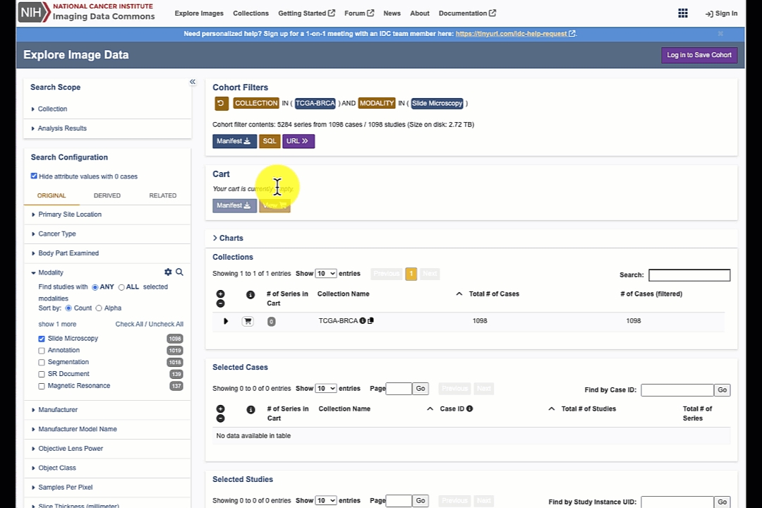
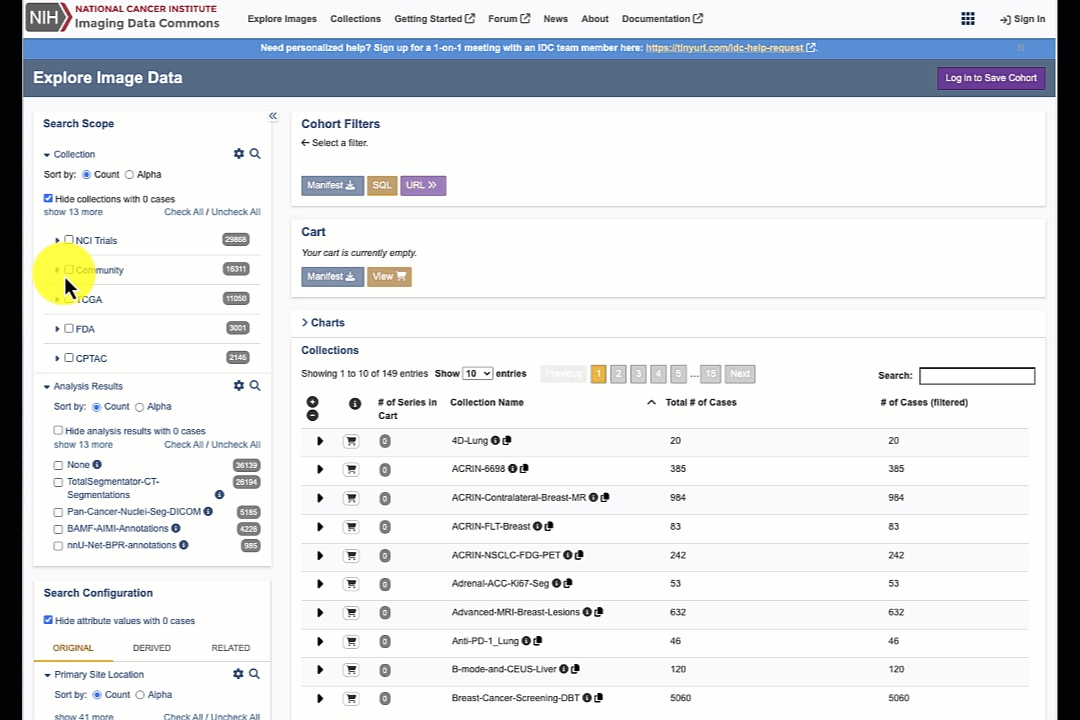
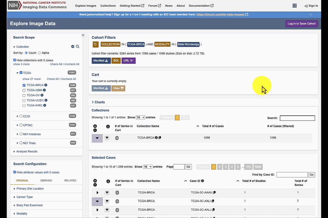


Categorical Numeric An attribute with data type Categorical Numeric has one of a defined set of numeric values. The corresponding value array must have a single numeric value. The (attribute, value array) pair for a Categorical Numeric is satisfied if the attribute is equal to the value in the value array. The /filters/values/{filter} endpoint returns a list of the values accepted for a Categorical Numeric attribute (filter).
Ranged Integer An attribute with data type Ranged Integer will have an integer value. For example, age_at_diagnosis is an attribute of data type Ranged Integer. In order to enable relative numeric queries, the API exposes eight variations of each Ranged Integer attribute as filter attribute names. These variations are the base attribute name with one of the suffixes: eq, gt, gte, btw, btwe, ebtw, ebtwe, lte, or lt, e.g. age_at_diagnosis_eq. The value array of the btw, btwe, ebtw, and ebtwe variations must contain exactly two integer values, in numeric order (least value first). The value array of the eq, gt, gte, lte, and lt variations must contain exactly one integer values. The (attribute, value array) pair for a Ranged Integer attribute is satisfied according to the suffix as follows:
eq: If an attribute is equal to the value in the value array
gt: If an attribute is greater than the value in the value array
gte: If an attribute is greater than or equal to the value in the value array
btw: if an attribute
Ranged Number An attribute with data type Ranged Number will have a numeric (integer or float) value. For example, diameter is an attribute of data type Ranged Number. In order to enable relative numeric queries, the API exposes eight variations of each Ranged Number attribute as filter attribute names. These variations are the base attribute name with one of the suffixes: eq, gt, gte, btw, btwe, ebtw, ebtwe, lte, or lt, e.g. diameter_eq. The value array of the btw, btwe, ebtw, and ebtwe variations must contain exactly two numeric values, in numeric order (least value first). The value array of the eq, gt, gte, lte, and lt variations must contain exactly one numeric values. The (attribute, value array) pair for a Ranged Number attribute is satisfied according to the suffix as follows:
eq: If an attribute is equal to the value in the value array
gt: If an attribute is greater than the value in the value array
gte: If an attribute is greater than or equal to the value in the value array
Detailed information on the DICOMweb endpoints that are available to access IDC data is provided here. In brief, there are two DICOM stores available - the IDC-maintained DICOM store and the Google-maintained DICOM store - we recommend that you familiarize yourself with the documentation to learn about the differences between the two, and select the option that is optimal for your use case.
Code snippets included in this article are also replicated in this Google Colab tutorial notebook for your convenience.
IDC uses DICOM for data organization, and every image contains metadata organized following the data model documented here. Each slide corresponds to a DICOM Series, uniquely identified by the SeriesInstanceUID, which in turn belongs to a DICOM Study identified by the StudyInstanceUID. You will need these two identifiers to access any DICOM slide using DICOMweb!
Since IDC contains many terabytes of images, you will typically want to first select images/slides that meet your needs. IDC offers various interfaces to explore and subset the data, starting from the IDC Portal, to the Python package idc-index (covered in this tutorial) and BigQuery SQL interfaces (see this tutorial). We strongly recommend you work through the referenced tutorials, but for the purposes of this tutorial, we will demonstrate how you can locate UIDs of a slide that corresponds to pancreas tissue.
First, install idc-index with pip install —upgrade idc-index (--upgrade part is very important to make sure you are working with the latest data release of IDC!).
Next, the following snippet demonstrates how to select slides of pancreas tissue (you can also select by the lens magnification, stain, and many other attributes - see this tutorial for details).
Next, we select the first slide and will use its StudyInstanceUID and SeriesInstanceUID in the subsequent sections of the code.
('2.25.25332367070577326639024635995523878122', '1.3.6.1.4.1.5962.99.1.3380245274.1362068963.1639762817818.2.0')
We recommend the following two Python libraries that facilitate access to a DICOM store via DICOMweb:
Both libraries can be installed using pip:
wsidicom is based upon the dicomweb_client Python library, while ez-wsi-dicomweb includes its own DICOMweb implementation.
Note that you can use wsidicom with both the IDC-maintained and the Google-maintained DICOM store, while ez-wsi-dicomweb only works with the Google-maintained store.
The following code snippets show exemplarily how to use each of the libraries to access a subregion from a DICOM slide identified by the following UIDs we selected earlier:
sample_study_uid = 2.25.25332367070577326639024635995523878122
sample_series_uid = 1.3.6.1.4.1.5962.99.1.3380245274.1362068963.1639762817818.2.0
When you work with wsidicom, the first step requires setting up dicomweb_client’s DICOMwebClient:
If you are accessing the Google-maintained DICOM store, you need to authenticate with your Google credentials first and set up an authorized session for the DICOMwebClient.
As discussed in the corresponding documentation page we mentioned earlier, Google-hosted DICOM store may not contain the latest version of IDC data! You will encounter access issues for slides that are not present. If this the case, you will need to use the IDC-hosted DICOM store instead!
Otherwise, if you prefer using IDC-maintained proxied DICOM store, you can skip ahead and just set up your DICOMwebClient using the proxy URL.
You now need to wrap the previously set-up DICOMwebClient into wsidicom’s WsiDicomWebClient. Then you can use the open_web() functionality to find, open and navigate the content of the selected slide:
To access a certain part of a slide, wsidicom offers the read_region() functionality:
The following code shows how to set-up an interface for DICOMweb with ez-wsi-dicomweb. You can only use this interface for accessing data from the Google-maintained DICOM store, which means authentication with you Google account is required.
The slide, slide level information and slide regions can be accessed as follows. To accelerate image retrieval, ez-wsi-dicomweb can be configured to fetch frames in blocks and cache them for subsequent use. For more information, check out this notebook, section “Enabling EZ-WSI DICOMweb Frame Cache”.
To iterate over image tiles you can simply wrap the functionality presented above into your own function that iterates over the coordinates of interest to you. In case you prefer to iterate over the frames as they are stored within the DICOM file, wsidicom does also offer a read_tile() method.
Iteration over a slide and accessing tiles from an area defined by a tissue mask can be quite easily achieved using ez-wsi-dicomweb’s DICOMPatchGenerator as described in this notebook in section “Generating patches from a level image”.
Both libraries — ez-wsi-dicomweb and wsidicom— can be recommended for reliable DICOMweb access to IDC data. Based on our experience, ez-wsi-dicomweb is often faster, likely due to its caching capabilities, and customizations for efficient access to image patches from a Google DICOM store for AI model training. wsidicom, on the other hand, is a more general-purpose tool offering extensive functionality for accessing DICOM files (images as well as annotation files) both from local disk or from the cloud via DICOMweb. It is important to note that when running code locally, access times may be slightly longer compared to cloud-based (such as in a Colab notebook) execution.
Over time, the set of data hosted by the IDC will change. For the most part, such changes will be due to new data having been added. The totality of IDC hosted data resulting from any such change is represented by a unique IDC data version ID. That is, each time that the set of publicly available data changes, a new IDC version is created that exactly defines the revised data set.
The IDC data version is intended to enable the reproducibility of research results. For example, consider a patient in the DICOM data model. Over time, new studies might be performed on a patient and become associated with that patient, and the corresponding DICOM instances will then be added to the IDC hosted data. Moreover, additional patients might well be added to the IDC data set over time. This means that the set of subjects defined by some filtering operation will change over time. Thus, for purposes of reproducibility, we define a cohort in terms of a set of filter groups and an IDC data version.
Note that on occasion some data might be removed from a collection, though this is expected to be rare. Such a removal will result in a new IDC data version which excludes that data. Such removed data will, however, continue to be available in any previous IDC data version in which it was available. There is one exception: data that is found to contain Personally Identifiable Information (PII) or Protected Health Information (PHI) will be removed from all IDC data versions.
Note: currently a cohort is always defined in terms of a single filter group and an IDC Data Version. In the future we may add support for multiple filter groups.
A filter group selects some set of subjects in the IDC hosted data, and is a set of conditions, where each condition is defined by an attribute and an array of values. An attribute identifies a field (column) in some data source (BQ table). Each filter group also specifies the IDC data version upon which it operates.
A filter group selects a subject if, for every attribute in the filter group, some datum associated with the subject satisfies one or more of the values in the associated array of values. A datum satisfies a value if it is equal to, less than, less than or equal to, between, greater than or equal to, or greater than, as required by the attribute. This is explained further below.
For example, the (attribute, [values]) pair (Modality, [MR, CT]) is satisfied if a subject "has" a Modality of MR or CT in any data associated with that subject. Thus, this (attribute, [values]) pair would be satisfied, for example, by a subject who has one or more MR series but no CT series.
Note that if a filter group includes more than one (attribute, [values]) pair having the same attribute, then only the last such (attribute, [values]) pair is used. Thus if a filter group includes the (attribute, [values]) pairs (Modality, [MR]) and (Modality, [CT]), in that order, only (Modality, [CT]) is used.
Here is an example filter group:
This filter group will select any subject in the TCGA-LUAD or TCGA-KIRC collections, if the subject has any DICOM instances having a modality of CT or MR, the subject's race is WHITE, and the subjects age at diagnosis is between 53 and 69.
A collection is a set of DICOM data provided by a single source. Collections are further categorized as Original collections or Analysis collections. Original collections are comprised primarily of DICOM image data that was obtained from some set of patients. Typically, the patients in an Original collection are related by a common disease.
Analysis collections are comprised of DICOM data that was generated by analyzing other (typically Original) collections. Typically such analysis is performed by a different entity than that which provided the original collection(s) on which the analysis is based. Examples of data in analysis collections include segmentations, annotations and further processing of original images. Note that some Original collections include such data, though most of the data in Original collections are original images.
A data source is a BQ table that contains some part of the IDC metadata complement. API queries are performed against one or more such tables that are joined (in the relational database model sense). Data sources are classified as being of type Original, Derived or Related. Original data sources contain DICOM metadata from the DICOM objects in TCIA Original and TCIA Analysis collections. Derived data sources contain processed data: in general this is analytical data has been processed to enable easier SQL searches. Related data sources contain ancillary data that may be specific to some set of collections. For example, TCGA biospecimen and clinical data are maintained in such tables.
Data sources are versioned. That is, when the data in a data source changes, a new version of that set of data is defined. An IDC data version is defined in terms of a specific version of each data source. Note that over time, new data sources may be added (or, less likely, removed). Thus two IDC data versions may have a different number of data sources.
Both the IDC Web App and API expose selected fields in the various data sources against which queries can be performed. Each attribute has a data type, one of:
String An attribute with data type String may have an arbitrary string value. For example, the possible values of a StudyDescription attribute are arbitrary. When the values array of a (String attribute, [values]) pair contains a single value, an SQL LIKE operator is used and standard SQL syntax and semantics are supported. Thus a ('StudyDescription",["%SKULL%"]) will match any StudyDescription that contains "SKULL", When the values array of a (String attribute, [values]) pair contains more that one value, an SQL UNNEST operator is used and standard SQL syntax and semantics are supported. See the Google BigQuery documentation for details.
Categorical String An attribute with data type Categorical String will have one of a defined set of string values. For example, Modality is an attribute, and has possible values 'CT', 'MR', 'SR', etc. In this case, the values are defined by the DICOM specification. The defined values of other Categorical String attributes may be established by other entities. When the values array of a (Categorical String attribute, [values]) pair contains a single value, an SQL LIKE operator is used and standard SQL syntax and semantics are supported. Thus a ('StudyDescription",["%SKULL%"]) will match any StudyDescription that contains "SKULL", When the values array of a (Categorical String attribute, [values]) pair contains more that one value, an SQL UNNEST operator is used and standard SQL syntax and semantics are supported. See the documentation for details.
Continuous Numeric An attribute with data type Continuous Number will have a numeric (float) value. For example, age_at_diagnosis is an attribute of data type Continuous Numeric. In order to enable relative numeric queries, the API exposes 6 variations of each Continuous Numeric attributes as filter set attribute names. These variations are the base attribute name with no suffix, as well as the base attribute name with one of the suffixes: _gt, _gte, _btw, _btwe, _ebtw, _ebtwe, _lte, _lt. The value array of the _*btw* variations must contain exactly two numeric values, in numeric order (least value first). The value array of the other variations must contain exactly one numeric values. The (attribute, value array) pair for a Continuous Numeric _attribute_ is satisfied according to the suffix as follows:
Categorical Numeric An attribute with data type Categorical Numeric has one of a defined set of numeric values. The corresponding value array must have a single numeric value.
A manifest is a list of access methods and other metadata of the data objects corresponding to the objects in some cohort. There are two types of access methods:
GUID
A GUID is a persistent identifier that can be resolved to a GA4GH DRS object. GUID persistence ensures that the data which the GUID represents can continue to be located and accessed even if it has been moved to a different hosting site. A GUID identifies a particular version of an IDC data object, and there is a GUID for every version of every DICOM instance and series in IDC hosted data. GUIDs are issued by the NCI Cancer Research Data Commons. This is a typical CRDC GUID: dg.4DFC/83fdfb25-ad87-4879-b0f3-b9850ef0b216 A GUID can be resolved at https://nci-crdc.datacommons.io/ga4gh/drs/v1/objects/ by appending the UUID to the that URL. E.G. (formatting added to the curl response for clarity):
>> curl https://nci-crdc.datacommons.io/ga4gh/drs/v1/objects/bd68332e-521f-4c45-9a88-e9cc426f5a8d
{ "access_methods":[{ "access_id":"gs", "access_url":{ "url":"gs://idc-open/bd68332e-521f-4c45-9a88-e9cc426f5a8d.dcm" }, "region":"", "type":"gs" } ], "aliases":[ ], "checksums":[ { "checksum":"9a63c81a4b3b4bc3950678a4e9acc930", "type":"md5" } ], "contents":[ ], "created_time":"2021-08-27T21:15:02.385181", "description":null, "form":"object", "id":"dg.4DFC/bd68332e-521f-4c45-9a88-e9cc426f5a8d", "mime_type":"application/json", "name":"", "self_uri":"drs://nci-crdc.datacommons.io/dg.4DFC/bd68332e-521f-4c45-9a88-e9cc426f5a8d", "size":528622, "updated_time":"2021-08-27T21:15:02.385185", "version":"faf7385b" }
Resolving such a GUID returns a DrsObject. The access methods in the returned DrsObject include one or more URLs at which corresponding DICOM entities can be accessed. GUID manifests are recommended for long term archival and reference.
In the above, we can see that the returned DrsObject includes the GCS URL gs://idc-open/bd68332e-521f-4c45-9a88-e9cc426f5a8d.dcm.
URL
The URLs in a URL based manifest can be used to directly access a DICOM instance in Google Cloud Storage. URLs are structured as follows:
gs://<GCS bucket>/<GUID>.dcm
This is a typical URL:
gs://idc-open/bd68332e-521f-4c45-9a88-e9cc426f5a8d.dcm
Though rare, the URL of some object can change over time. In such a case, the corresponding DRSObject will be updated with new URL. However, the original URL will then be "stale".
Additional values can optionally be included in the returned manifest. See the manifest API descriptions for more details.
The IDC API UI can be used to see details about the syntax for each call, and also provides an interface to test requests.
For a quick demonstration of the syntax of an API call, test the GET/collections request. You can experiment with this endpoint by clicking the ‘Try it out’ button.
The API will return collection metadata for the current IDC data version. The request can be run by selecting ‘Execute’.
Request Response
The Swagger UI submits the request and shows the curl code that was submitted. The ‘Response body’ section will display the response to the request. The expected format of the response to this API request is shown below:
The actual JSON formatted response can be downloaded by selecting the ‘Download’ button.
The syntax for all of API data structures is detailed at the bottom of the UI page.


The version of the portal is shown at the bottom of the portal page. The semantics of the version is the following:
canceridc.<date of webapp deployment in YYYYMMDDHHMM>.<first 6 characters of the commit hash>,
where revision hash corresponds to that of the .
Portal release notes are maintained at
{
"filters": {
"collection_id": [
"TCGA-LUAD",
"TCGA-KIRC"
],
"Modality": [
"CT",
"MR"
],
"race": [
"WHITE"
],
"age_at_diagnosis_btw": [
65,
75
]
}
}{
"collections": [
{
"cancer_type": "string",
"collection_id": "string",
"date_updated": "string",
"description": "string",
"doi": "string",
"image_types": "string",
"location": "string",
"species": "string",
"subject_count": 0,
"supporting_data": "string",
}
],
"code": 200
}from idc_index import IDCClient
# Instantiate the client
idc_client = IDCClient()
idc_client.fetch_index('sm_index')
# Filter the slides
query = """
SELECT index.StudyInstanceUID, sm_index.SeriesInstanceUID
FROM sm_index
JOIN index ON sm_index.SeriesInstanceUID = index.SeriesInstanceUID
WHERE Modality = 'SM' AND primaryAnatomicStructure_CodeMeaning = 'Pancreas'
"""
pancreas_slides = idc_client.sql_query(query)sample_study_uid = pancreas_slides['StudyInstanceUID'][0]
sample_series_uid = pancreas_slides['SeriesInstanceUID'][0]
sample_study_uid, sample_series_uidpip install wsidicom
pip install ez-wsi-dicomwebfrom dicomweb_client.api import DICOMwebClient
from dicomweb_client.ext.gcp.session_utils import create_session_from_gcp_credentialsfrom google.colab import auth
auth.authenticate_user()
# Create authorized session
session = create_session_from_gcp_credentials()
# Set-up a DICOMwebClient using the dicomweb_client library
google_dicom_store_url = 'https://healthcare.googleapis.com/v1/projects/nci-idc-data/locations/us-central1/datasets/idc/dicomStores/idc-store-v21/dicomWeb'
dw_client = DICOMwebClient(
url=dicom_store_url,
session=session
)# Set-up a DICOMwebClient using the dicomweb_client library
idc_dicom_store_url = 'https://proxy.imaging.datacommons.cancer.gov/current/viewer-only-no-downloads-see-tinyurl-dot-com-slash-3j3d9jyp/dicomWeb'
dw_client = DICOMwebClient(url=idc_dicom_store_url)import wsidicom
import matplotlib.pyplot as plt
wsidicom_client = wsidicom.WsiDicomWebClient(dw_client)
slide = wsidicom.WsiDicom.open_web(wsidicom_client,
study_uid=sample_study_uid,
series_uids=sample_series_uid
)
print(slide)[0]: Pyramid of levels:
[0]: Level: 0, size: Size(width=171359, height=74498) px, mpp: SizeMm(width=0.2472, height=0.2472) um/px Instances: [0]: default z: 0.0 default path: 1 ImageData <wsidicom.web.wsidicom_web_image_data.WsiDicomWebImageData object at 0x7d0f16444c50>
[1]: Level: 2, size: Size(width=42839, height=18624) px, mpp: SizeMm(width=0.988817311328, height=0.988817311328) um/px Instances: [0]: default z: 0.0 default path: 1 ImageData <wsidicom.web.wsidicom_web_image_data.WsiDicomWebImageData object at 0x7d0f16445410>
[2]: Level: 4, size: Size(width=10709, height=4656) px, mpp: SizeMm(width=3.955546250817, height=3.955546250817) um/px Instances: [0]: default z: 0.0 default path: 1 ImageData <wsidicom.web.wsidicom_web_image_data.WsiDicomWebImageData object at 0x7d0f165271d0>
[3]: Level: 6, size: Size(width=2677, height=1164) px, mpp: SizeMm(width=15.823662607396, height=15.823662607396) um/px Instances: [0]: default z: 0.0 default path: 1 ImageData <wsidicom.web.wsidicom_web_image_data.WsiDicomWebImageData object at 0x7d0f14192750># Access and visualize 500x500px subregion at level 4, starting from pixel (1000,1000)
region = slide.read_region(location=(1000, 1000), level=4, size=(500, 500))
plt.imshow(region)
plt.show()from ez_wsi_dicomweb import dicomweb_credential_factory
from ez_wsi_dicomweb import dicom_slide
from ez_wsi_dicomweb import local_dicom_slide_cache_types
from ez_wsi_dicomweb import dicom_web_interface
from ez_wsi_dicomweb import patch_generator
from ez_wsi_dicomweb import pixel_spacing
from ez_wsi_dicomweb.ml_toolkit import dicom_path
from google.colab import auth
auth.authenticate_user()
google_dicom_store_url = 'https://healthcare.googleapis.com/v1/projects/nci-idc-data/locations/us-central1/datasets/idc/dicomStores/idc-store-v20/dicomWeb'
series_path_str = (
f'{google_dicom_store_url}'
f'/studies/{sample_study_uid}'
f'/series/{sample_series_uid}'
)
series_path = dicom_path.FromString(series_path_str)
dcf = dicomweb_credential_factory.CredentialFactory()
dwi = dicom_web_interface.DicomWebInterface(dcf)ds = dicom_slide.DicomSlide(
dwi=dwi,
path=series_path,
enable_client_slide_frame_decompression = True
)
# More information: https://github.com/GoogleCloudPlatform/EZ-WSI-DICOMweb/blob/main/ez_wsi_demo.ipynb
ds.init_slide_frame_cache( optimization_hint=local_dicom_slide_cache_types.CacheConfigOptimizationHint.MINIMIZE_LATENCY
)# Investigate existing levels and their dimensions
for level in ds.levels:
print(f'Level {level.level_index} has pixel dimensions (row, col): {level.height, level.width}')Level 1 has pixel dimensions (row, col): (74498, 171359)
Level 2 has pixel dimensions (row, col): (18624, 42839)
Level 3 has pixel dimensions (row, col): (4656, 10709)
Level 4 has pixel dimensions (row, col): (1164, 2677)# Access and visualize 500x500px subregion at level 3, starting from pixel (1000,1000)
level = ds.get_level_by_index(3)
region = ds.get_patch(level=level, x=1000, y=1000, width=500, height=500).image_bytes()
plt.imshow(region)
plt.show() {
"idc_data_version": "1.0",
"filters": {
"collection_id": [
"TCGA-LUAD",
"TCGA-KIRC"
],
"Modality": [
"CT",
"MR"
],
"race": [
"WHITE"
],
"age_at_diagnosis_btw": [
53, 69
]
}{
"collections": [
{
"cancer_type": "string",
"collection_id": "string",
"date_updated": "string",
"description": "string",
"doi": "string",
"image_types": "string",
"location": "string",
"species": "string",
"subject_count": 0,
"supporting_data": "string",
}
],
"code": 200
}ebtw: if an attribute is greater than or equal to the first value and less than the second value in the value array
btwe: if an attribute is greater than the first value and less than or equal to the second value in the value array
ebtwe: if an attribute is greater than or equal to the first value and less than or equal to the second value in the value array
lte: If an attribute is less than or equal to the value in the value array
lt: If an attribute is less than the value in the value array
ebtw: if an attribute is greater than or equal to the first value and less than the second value in the value array
btwe: if an attribute is greater than the first value and less than or equal to the second value in the value array
ebtwe: if an attribute is greater than or equal to the first value and less than or equal to the second value in the value array
lte: If an attribute is less than or equal to the value in the value array
lt: If an attribute is less than the value in the value array
gt: If an attribute is greater than the value in the value array
gte: If an attribute is greater than or equal to the value in the value array
btw: if an attribute is gt the first value and lt the second value in the value array
ebtw: if an attribute is gte the first value and lt the second value in the value array
btwe: if an attribute is gt the first value and lte the second value in the value array
ebtwe: if an attribute is gte the first value and lte the second value in the value array
lte: If an attribute is less than or equal to the value in the value array
lt: If an attribute is less than the value in the value array

on the Explore Images page the IDC internal id for each collection can now be copied from the Collections table by clicking the corresponding copy icon
on the Explore Images page the IDC case id can now be copied from the Selected Cases table by clicking the corresponding copy icon
Main highlights of this release include:
add a choice of several viewers (OHIF v2, OHIF v3, VolView, Slim) for viewing image files
Main highlights of this release include:
s5cmd file manifests can now be generated from the Explore images page for individual studies and series
Main highlights of this release include:
The file manifest for a filter can be downloaded without logging into the portal and creating a persistent cohort
Main highlights of this release include:
The Export Cohort Manifest popup now includes options to download manifests that can be used by s5cmd to download image files from IDC's s3 buckets in GCP or AWS. Instructions are provided for using s5cmd with these manifests
Main highlights of this release include:
Three new Original Image attributes Max Total Pixel Matrix Columns, Max Total Pixel Matrix Rows, and Min Pixel Spacing are added.
Two new Quantitative Analysis attributes Sphericity (Quant) and Volume of Mesh are added.
Default attribute value order is changed from alphanumeric (by value name) to value count.
Main highlights of this release include:
As limited access collections have been removed from IDC, the portal is now simplified by removing the option of selecting different access levels. All collections in the portal are public.
A warning message appears on the cohort browser page when a user views a cohort that used the Access filter attribute. That attribute is no longer applied if the user migrates the cohort to the current version.
On the explorer page the reset button has been moved to improve viewability.
This was primarily a data release. There were no significant changes to the portal.
Main highlights of this release include:
User control over how selection of multiple filter modalities defines the cohort. Previously when multiple modalities were selected the cohort would include the cases that had ANY of the selected modalities. Now the user can choose if the cohort includes the cases that contain ANY of the selected modaltiies or just those that have ALL of the selected modalities.
Main highlights of this release include:
Ability to select specific Analysis Results collections with segmentation and radiomic features
Text boxes added to the slider panels to allow the user to input upper and lower slider bounds
Pie chart tooltips updated to improve viewability
Main highlights of this release include:
Eleven new collections added
Number of cases, studies, and series in a cohort are reported in the filter de finition
On the Exploration page the Access attribute is placed in the Search Scope
On the Exploration page users are warned when they create a cohort that includes Limited Access collections
Series Instance UID is reported in the Selected Series table
Main highlights of this release include:
The BigQuery query string corresponding to a cohort can now be displayed in user-readable format by pressing a button on either the cohort or cohort list pages
On the exploration page collections can now be sorted alphabetically or by the number of cases. Selected cases are ordered at the top of the collection list
Table rows can be selected by clicking anywhere within the row, not just on the checkbox
The BigQuery export cohort manifest includes the IDC data version as an optional column
Main highlights of this release include:
Collections which have limited access are now denoted as such in the Collection tab on the Exploration page
Links to image files belonging to limited collections have been removed from the Studies and Series tables on the Exploration page
The quota of image file data that can be served per user per day has been reduced from 137 to 40 GB
Main highlights of this release include:
New attributes including Manufacturer, Manufacturer Model Name, and Slice Thickness added
Checked attribute values are now shown at the top of the attribute value lists
Ability to search by CaseID added to the Selected Cases table
Ability to search by StudyID added to the Selected Studies table
Study Date added to the Studies Table
Changed the persistence of the StudyID tooltip in the tables so that the StudyID can be copied from the tooltip
Specific columns can now be selected in the BigQuery cohort export
The Imaging Data Commons Explore Image Data portal is a platform that allows users to explore, filter, create cohorts, and view image studies and series using cutting-edge technology viewers.
Main highlights of this release include:
Support for slide microscopy series from the CPTAC-LSCC and CPTAC-LUAD collections is now included.
The Slim viewer is now configured to view slide microscopy series
Search boxes are included for very attribute to search for specific attribute values by name.
The Imaging Data Commons Explore Image Data portal is a platform that allows users to explore, filter, create cohorts, and view image studies and series using cutting-edge technology viewers.
Main highlights of this release include:
112 data collections are now included
Cohort data version is reported
Cohort statistics - ie the number the cases, studies, and series per cohort are now reported
Mechanism included to update a version cohort
Species Attribute is included
Checkbox and plus/minus icons are now used to select table rows
The Imaging Data Commons Explore Image Data portal is a platform that allows users to explore, filter, create cohorts, and view image studies and series using cutting-edge technology viewers.
Main highlights of this release include:
The user details page will no longer return a 500 error when selected
Sorting of studies panel is now active for all fields
Re-sending of an unreceived verification email is now more clearly explained.
IDC identity login header and column selection is disabled for the exportation of a cohort manifest to BigQuery
Detailed information panel added to efficiently describe why some pie charts have multiple facets even when a filter is selected
Cohort manifest export popup can be scrolled down
Use of Shift or Control (Command for Mac) selection of studies will now behave as expected: Shift-select for a contiguous series of rows, Control/Command-select for individual rows.
All filter selections are now sorted by alphabetical characters
The Imaging Data Commons Explore Image Data portal is a platform that allows users to explore, filter, create cohorts, and view image studies and series using cutting-edge technology viewers.
Main highlights of this release include:
Consistent number of files will be returned between the portal and BigQuery
When the user clicks a non-gov link a popup will appear
Cohort manifest export information now has clickable URLs to take you to the BigQuery console
Collections list displays by default 100 entries
Any empty search criteria is now highlighted in grey and no data will be listed
The user will no longer need to scroll to see search criteria in the left search configuration panel
Portal footer is now in compliance with NCI requirements
Check/uncheck in the collections panel added for collection TCGA
The Imaging Data Commons Explore Image Data portal is a platform that allows users to explore, filter, create cohorts, and view image studies and series using cutting-edge technology viewers.
Main highlights of this release include:
Case-level table is added to the portal
Cohorts can now be exported into BigQuery tables using the Export Cohort Manifest button
Cohorts less than 650k rows can now be downloaded as a multipart file. Cohorts larger that 600k rows can only be be exported to BigQuery (for users that are logged in with Google Accounts)
Quantitative filter ranges are updated dynamically with the updates to filter selection
Pie charts will display "No data available" message when zero cases are returned for the given filter selection
RTPLAN and Real World Mapping Attribute values are now disabled at the series level, since they cannot be visualized in the IDC Viewer
Various bug fixes in both the IDC Portal and IDC Viewer
The Imaging Data Commons Explore Image Data portal is a platform that allows users to explore, filter, create cohorts, and view image studies and series using cutting-edge technology viewers.
Main features in this initial release include:
The ability to search for data in BigQuery and Solr
The ability to search by multiple attributes:
Collection
Original attributes e.g., Modality
Derived attributes e.g., Segmentations
Qualitative analysis e.g., Lobular pattern
Quantitative analysis e.g., Volume
related attributes e.g., Country
Display of collections results in a tabular format with the following information:
Collection Name
Total Number of Cases
Number of Cases(this cohort)
Display of the Selected Studies results in tabular format with the following information:
Project Name
Case ID
Study ID
Display of the Selected Series results in tabular format with the following information:
Study ID
Series Number
Modality
The ability to hide attributes with zero cases present
The ability to save cohorts
The ability to download the manifest of any cohort created
The ability to promote, filter, and load multiple series instances in the OHIF viewer


Study Description
Body Part Examined
Series Description

BQ tables are organized in BQ datasets. BQ datasets are not unlike folders on your computer, but contain tables related to each other instead of files. BQ datasets, in turn, are organized under Google Cloud projects. GCP projects can be thought of as containers that are managed by a particular organization. To continue with the file system analogy, think about projects as hard drives that contain folders.
This may be a good time for you to complete Part 1 of the IDC "Getting started" tutorial series, so that you are able to open the tables and datasets we will be discussing in the following paragraphs!
Let's map the aforementioned project-dataset-table hierarchy to the concrete locations that contain IDC data.
All of the IDC tables are stored under the bigquery-public-data project. That project is managed by Google Public Datasets Program, and contains many public BQ datasets, beyond those maintained by IDC.
All of the IDC tables are organized into datasets by data release version. If you complete the tutorial mentioned above, open the BQ console, and scroll down the list of datasets, you will find those that are named starting with the idc_v prefix - those are IDC datasets.
Following the prefix, you will find the number that corresponds to the IDC data release version. IDC data releases version numbers start from 1 and are incremented by one for each subsequent release. As of writing this, the most recent version of IDC is 16, and you can find dataset idc_v16 corresponding to this version.
In addition to idc_v16 you will find a dataset named idc_v16_clinical. That dataset contains clinical data accompanying IDC collections. We started clinical data ingestion in IDC v11. If you want to learn more about the organization and searching of clinical data, take a look at the .
Finally, you will also see two special datasets: idc_current and idc_current_clinical. Those two datasets are essentially aliases, or links, to the versioned datasets corresponding to the latest release of IDC data.
If you want to explore the latest content of IDC - use current datasets.
If you want to make sure your queries and data selection are reproducible - always use the version numbered datasets!
Before we dive into discussing the individual tables maintained by IDC, there is just one more BigQuery-specific concept you need to learn: the view. BigQuery view is a table that is defined by an SQL query that is run every time you query the view (you can read more about BQ views in ).
BQ views can be very handy when you want to simplify your queries by factoring out the part of the query that is often reused. But a key disadvantage of BQ views over tables is the reduced performance and increased cost due to re-running the query each time you query the view.
As we will discuss further, most of the tables maintained by IDC are created by joining and/or post-processing other tables. Because of this we rely heavily on BQ views to improve transparency of the provenance of those "derived" tables. BQ views can be easily distinguished from the tables in a given dataset by a different icon. IDC datasets also follow a convention that all views in the versioned datasets include suffix _view in the name, and are accompanied by the result of running the query used by the view in a table that has the same name sans the _view suffix. See the figure below for an illustration of this convention.
If you are ever curious (and you should be, at least once in a while!) about the queries behind individual views, you can click on the view in the BQ console, and see the query in the "Details" tab. Try this out yourself to check the query for
Now that we reviewed the main concepts behind IDC tables organization, it is time to explain the sources of metadata contained in those tables. Leaving _clinical datasets aside, IDC tables are populated from one of the two sources:
DICOM metadata extracted from the DICOM files hosted by IDC, and various derivative tables that simplify access to specific DICOM metadata items;
collection-level and auxiliary metadata, which is not stored in DICOM tags, but is either received by IDC from other sources, or is populated by IDC as part of data curation (these include Digital Object Identifiers, description of the collections, hashsums, etc).
The set of BQ tables and views has grown over time. The enumeration below documents the BQ tables and views as of IDC v14. Some of these tables will not be found in earlier IDC BigQuery datasets.
dicom_metadataEach row in the dicom_metadata table holds the DICOM metadata of an instance in the corresponding IDC version. There is a single row for each DICOM instance in the corresponding IDC version, and the columns correspond to the DICOM attributes encountered in the data across all of the ingested instances.
IDC utilizes the standard capabilities of the Google Healthcare API to extract all of the DICOM metadata from the hosted collections into a single BQ table. Conventions of how DICOM attributes of various types are converted into BQ form are covered in the Google Healthcare API documentation article.
dicom_metadata table contains DICOM metadata extract from the files included in the given IDC data release. The amount and variety of the DICOM files grows with the new releases, and the schema of this table reflects the organization of the metadata in each IDC release. Non-sequence attributes, such as Modality or SeriesInstanceUID, once encountered in any one file will result in the corresponding column being introduced to the table schema (i.e., if we have column X in IDC release 11, in all likelihood it will also be present in all of the subsequent releases).
Sequence DICOM attributes, however, may have content that is highly variable across different DICOM instances (especially in Structured Reports). Those attributes will map to , and it is not unusual to see drastic differences in the corresponding columns of the table between different releases.
dicom_metadata can be used to conduct detailed explorations of the metadata content, and build cohorts using fine-grained controls not accessible from the IDC portal. Note that the dicom_all table, described below, is probably a better choice for such explorations.
Due to the existing limitations of Google Healthcare API, not all of the DICOM attributes are extracted and are available in BigQuery tables. Specifically:
sequences that have more than 15 levels of nesting are not extracted (see ) - we believe this limitation does not affect the data stored in IDC
sequences that contain around 1MiB of data are dropped from BigQuery export and RetrieveMetadata output currently. 1MiB is not an exact limit, but it can be used as a rough estimate of whether or not the API will drop the tag (this limitation was not documented as of writing this) - we know that some of the instances in IDC will be affected by this limitation. The fix for this limitation is targeted for sometime in 2021, according to the communication with Google Healthcare support.
auxiliary_metadataThis table defines the contents of the corresponding IDC version. There is a row for each instance in the version. We group the attributes for convenience:
Collection attributes:
tcia_api_collection_id: The ID, as accepted by the TCIA API, of the original data collection containing this instance (will be Null for collections not sourced from TCIA)
idc_webapp_collection_id: The ID, as accepted by the IDC web app, of the original data collection containing this instance
collection_id: The ID, as accepted by the IDC web app. Duplicate of idc_webapp_collection_id
Patient attributes:
submitter_case_id:The Patient ID assigned by the submitter of this data. This is the same as the DICOM PatientID
idc_case_id:IDC generated UUID that uniquely identifies the patient containing this instance
This is needed because DICOM PatientIDs are not required to be globally unique
patient_hash: md5 hash of this version of the patient/case containing this instance
Study attributes:
StudyInstanceUID: DICOM UID of the study containing this instance
study_uuid:IDC assigned UUID that identifies a version the the study containing this instance.
study_instances: The number instances in the study containing this instance
Series attributes:
SeriesInstanceUID: DICOM UID of the series containing this instance
series_uuid:IDC assigned UUID that identifies the version of the series containing this instance
source_doi:The DOI of an information page corresponding to the original data collection or analysis results that is the source of this instance
Instance attributes:
SOPInstanceUID: DICOM UID of this instance.
instance_uuid:IDC assigned UUID that identifies the version of this instance.
gcs_url: The GCS URL of a file containing the version of this instance that is identified by this series_uuid/instance_uuid
mutable_metadataSome non-DICOM metadata may change over time. This includes the GCS and AWS URLs of instance data, the accessibility of each instance and the URL of an instance's associated description page. BigQuery metadata tables such as the auxiliary_metadata and dicom_all tables are never revised even when such metadata changes. However, tables in the datasets of previous IDC versions can be joined with the mutable_metadata table to obtain the current values of these mutable attributes.
The table has one row for each version of each instances:
crdc_instance_uuid: The uuid of an instance version
crdc_series_uuid: The uuid of a series version that contains this instance version
crdc_study_uuid: The uuid of a study version that contains the series version
original_collections_metadataThis table is comprised of IDC data collection-level metadata for the original TCIA data collections hosted by IDC, for the most part corresponding to the content available in . One row per collection:
tcia_api_collection_id: The collection ID as is accepted by the TCIA AP
tcia_wiki_collection_id: The collection ID as on the TCIA wiki page
idc_webapp_collection_id:The collection ID as accepted by the IDC web app
analysis_results_metadataMetadata for the TCIA analysis results hosted by IDC, for the most part corresponding to the content available in . One row per analysis result:
ID: Results ID
Title: Descriptive title
DOI:DOI that can be resolved at doi.org to the TCIA wiki page for this analysis result
version_metadataMetadata for each IDC version, one row per version:
idc_version: IDC version number
version_hash: MD5 hash of hashes of collections in this version
version_timestamp: Version creation timestamp
The following tables and views consist of metadata derived from one or more other IDC tables tables for convenience of the user. For each such table, <table_name>, there is also a corresponding view, <table_name>_view, that, when queried, generates an equivalent table. These views are intended as a reference; each view's SQL is available to be used for further investigation.
Several of these tables/views are discussed more completely .
dicom_all, dicom_all_viewAll columns from dicom_metadata together with selected date from the auxiliary_metadata, original_collections_metadata, and analysis_results_metadata tables.
segmentations, segmentations_viewThis table is derived from dicom_all to simplify access to the attributes of DICOM Segmentation objects available in IDC. Each row in this table corresponds to one DICOM Segmentation instance segment.
measurement_groups, measurement_groups_viewThis table is derived from dicom_all to simplify access to the measurement groups encoded in DICOM Structured Report TID 1500 objects available in IDC. Specifically, this table contains measurement groups corresponding to the "Measurement group" content item in the DICOM SR objects.
Each row corresponds to one TID1500 measurement group.
qualitative_measurements, qualitative_measurements_viewThis table is derived from dicom_all to simplify access to the qualitative measurements in DICOM SR TID1500 objects. It contains coded evaluation results extracted from the DICOM SR TID1500 objects. Each row in this table corresponds to a single qualitative measurement extracted.
quantitative_measurements, quantitative_measurements_viewThis table is derived from dicom_all to simplify access to the quantitative measurements in DICOM SR TID1500 objects. It contains quantitative evaluation results extracted from the DICOM SR TID1500 objects. Each row in this table corresponds to a single quantitative measurement extracted.
dicom_metadata_curated, dicom_metadata_curated_viewCurated values of DICOM metadata extracted from dicom_metadata.
dicom_metadata_curated_series_level, dicom_metadata_curated_series_level_viewCurated columns from dicom_metadata that have been aggregated/cleaned up to describe content at the series level. Each row in this table corresponds to a DICOM instance in IDC. The columns are curated by defining queries that apply transformations to the original values of DICOM attributes.
idc_pivot_v<idc version>A view that is the basis for the queries performed by the IDC web app.
Most clinical data is found in the . However, a few tables of clinical data are found in the idc_v<idc_version> datasets.
The following tables contain TCGA-specific metadata:
tcga_biospecimen_rel9: biospecimen metadata
tcga_clinical_rel9: clinical metadata
The following tables contain NLST specific metadata. The detailed schema of those tables is available from the .
nlst_canc: "Lung Cancer"
nlst_ctab: "SCT Abnormalities"
nlst_ctabc: "SCT Comparison Abnormalities"
DICOM files in the IDC are stored as "blobs" on the cloud, with one copy housed on Google Cloud Storage (GCS) and another on Amazon Web Services (AWS) S3 storage. By using the right tools, these blobs can be wrapped to appear as "file-like" objects to Python DICOM libraries, enabling intelligent loading of DICOM files directly from cloud storage as if they were local files without having to first download them onto a local drive.
Code snippets included in this article are also replicated in this Google Colab tutorial notebook for you convenience:
collection_timestamp: Datetime when the IDC data in the collection was last revised
collection_hash: md5 hash of the of this version of the collection containing this instance
collection_init_idc_version: The IDC version in which the collection containing this instance first appeared
collection_revised_idc_version: The IDC version in which this version of the collection containing this instance first appeared
patient_init_idc_version: The IDC version in which the patient containing this instance first appeared
patient_revised_idc_version: The IDC version in which this version of the patient/case containing this instance first appeared
study_hash: md5 hash of the data in this version of the study containing this instance
study_init_idc_version: The IDC version in which the study containing this instance first appeared
study_revised_idc_version: The IDC version in which this version of the study containing this instance first appeared
source_url:The URL of an information page that describes the original collection or analysis result that is the source of this instance
series_instances: The number of instances in the series containing this instance
series_hash: md5 hash of the data in the this version of the series containing this instance
access: Collection access status: 'Public' or 'Limited'. (Currently all data is 'Public')
series_init_idc_version: The IDC version in which the series containing this instance first appeared
series_revised_idc_version: The IDC version in which this version of the series containing this instance first appeared
aws_url: The AWS URL of a file containing the version of this instance that is identified by this series_uuid/instance_uuid
instance_hash: the md5 hash of this version of this instance
instance_size: the size, in bytes, of this version of this instance
instance_init_idc_version: The IDC version in which this instance first appeared
instance_revised_idc_version: The IDC version in which this version of this instance first appeared
license_url: The URL of a web page that describes the license governing this version of this instance
license_long_name: A long form name of the license governing this version of this instance
license_short_name: A short form name of the license governing this version of this instance
gcs_url: URL to the Google Cloud Storage (GCS) object containing this instance versionaws_url: URL to the Amazon Web Services (AWS) object containing this instance version
`access: Current access status of this instance (Public or Limited)
source_url: The URL of a page that describes the original collection or analysis result that includes this instance
source_doi: The DOI of a page that describes the original collection or analysis result that includes this instance
Program: The program to which this collection belongsUpdated: Most recent update date reported by the collection source
Status:Collection status: "Ongoing" or "Complete"
Access:Collection access conditions: "Limited" or "Public"
ImageType: Enumeration of image types/modalities in the collection
Subjects:Number of subjects in the collection
DOI:DOI that can be resolved at doi.org to the TCIA wiki page for this collection
URL:URL of an information page for this collection
CancerType:Collection source(s) assigned cancer type of this collection
SupportingData:Type(s) of additional data available
Species: Species of collection subjects
Location:Body location that was studied
Description: Description of the collection (HTML format)
license_url: The URL of a web page that describes the license governing this collection
license_long_name: A long form name of the license governing this collection
license_short_name: A short form name of the license governing this collection
CancerType:TCIA assigned cancer type of this analysis resultLocation:Body location that was studied
Subjects:Number of subjects in the analysis result
Collections: Original collections studied
AnalysisArtifactsonTCIA: Type(s) of analysis artifacts generated
Updated: Data when results were last updated
license_url: The URL of a web page that describes the license governing this collection
license_long_name: A long form name of the license governing this collection
license_short_name: A short form name of the license governing this collection
description: Description of analysis result
nlst_prsn: "Participant"nlst_screen: "SCT Screening"


dicom_all_view is a BQ view, as indicated by the icon to the left from the table name. dicom_all table is the result of running the query that defines the dicom_all_view. 
Pydicom is popular library for working with DICOM files in Python. Its dcmread function is able to accept any "file-like" object, meaning you can read a file straight from a cloud blob if you know its path. See this page for information on finding the paths of the blobs for DICOM objects in IDC. The dcmread function also has some other options that allow you to control what is read. For example you can choose to read only the metadata and not the pixel data, or read only certain attributes. In the following two sections, we demonstrate these abilities using first Google Cloud Storage blobs and then AWS S3 blobs.
Mapping IDC DICOM series to bucket URLs
All of the image data available from IDC is replicated between public Google Cloud Storage (GCS) and AWS buckets. pip-installable idc-index package provides convenience functions to get URLs of the files corresponding to a given DICOM series.
From Google Cloud Storage blobs
The official Python SDK for Google Cloud Storage (installable from pip and PyPI as google-cloud-storage) provides a "file-like" interface allowing other Python libraries, such as Pydicom, to work with blobs as if they were "normal" files on the local filesystem.
To read from a GCS blob with Pydicom, first create a storage client and blob object, representing a remote blob object stored on the cloud, then simply use the .open('rb') method to create a readable file-like object that can be passed to the dcmread function.
Reading only metadata or only specific attributes will reduce the amount of data that needs to be pulled down under some circumstances and therefore make the loading process faster. This depends on the size of the attributes being retrieved, the chunk_size (a parameter of the open() method that controls how much data is pulled in each HTTP request to the server), and the position of the requested element within the file (since it is necessary to seek through the file until the requested attributes are found, but any data after the requested attributes need not be pulled). If you are not retrieving entire images, we strongly recommend specifying a chunk_size (in bytes) because the default value is around 40MB, which is typically far larger than the optimal value for accessing metadata attributes or individual frames (see later).
This works because running the open method on a Blob object returns a BlobReader object, which has a "file-like" interface (specifically the seek, read, and tell methods).
From AWS S3 blobs
The s3fs package provides "file-like" interface for accessing S3 blobs. It can be installed with pip install s3fs. The following example repeats the above example using the counterpart of the same blob on AWS S3.
Similar to the chunk_size parameter in GCS, the default_block_size is crucially important for determining how efficient this is. Its default value is around 50MB, which will result in orders of magnitude more data than necessary being pulled than is needed to retrieve metadata. In the above example, we set it to 50kB.
Highdicom is a higher-level library providing several features to work with images and image-derived DICOM objects. As of the release 0.25.1, its various reading methods (including imread, segread, annread, and srread) can read any file-like object, including Google Cloud blobs and S3 blobs opened with s3fs.
A particularly useful feature when working with blobs is "lazy" frame retrieval for images and segmentations. This downloads only the image metadata when the file is initially loaded, uses it to create a frame-level index, and downloads specific frames as and when they are requested by the user. This is especially useful for large multiframe files (such as those found in slide microscopy or multi-segment binary or fractional segmentations) as it can significantly reduce the amount of data that needs to be downloaded to access a subset of the frames.
In this first example, we use lazy frame retrieval to load only a specific spatial patch from a large whole slide image from the IDC using GCS.
Running this code should produce an output that looks like this:
The next example repeats this on the same image in AWS S3:
In both cases, we set the chunk_size/default_block_size to around 500kB, which should be enough to ensure each frame can be retrieved in a single request while minimizing further unnecessary data retrieval.
As a further example, we use lazy frame retrieval to load only a specific set of segments from a large multi-organ segmentation of a CT image in the IDC stored in binary format (in binary segmentations, each segment is stored using a separate set of frames) using GCS.
See this page for more information on highdicom's Image class, and this page for the Segmentation class.
Achieving good performance for the Slide Microscopy frame-level retrievals requires the presence of either a "Basic Offset Table" or "Extended Offset Table" in the file. These tables specify the starting positions of each frame within the file's byte stream. Without an offset table being present, libraries such as highdicom have to parse through the pixel data to find markers that tell it where frame boundaries are, which involves pulling down significantly more data and is therefore very slow. This mostly eliminates the potential speed benefits of frame-level retrieval. Unfortunately there is no simple way to know whether a file has an offset table without downloading the pixel data and checking it. If you find that an image takes a long time to load initially, it is probably because highdicom is constucting the offset table itself because it wasn't included in the file.
Most IDC images do include an offset table, but some of the older pathology slide images do not. This page contains some notes about whether individual collections include offset tables.
You can also check whether an image file (including pixel data) has an offset table using pydicom like this:
To do this from a remote Google Cloud Storage blob without needing to pull all the pixel data, you can do something like this:
As discussed in this community forum post, TCIA made the decision to pull a subset of data from public access collections to limited access. At the moment, we still keep those files that used to be public in IDC before the decision made by TCIA, and the metadata for those files is still accessible in our BigQuery tables, but you cannot download those “Limited” access files referenced by gcs_url from IDC.
As discussed in this post the issue will manifest itself in an error accessing gcs_url that corresponds to a non-public file:
has a column named access , which takes values Public or Limited that define if the file corresponding to the instance can be accessed. For all practical purposes, if you interact with the IDC BigQuery tables, you should make sure you exclude “Limited” access items using the following clause in your query:
In a future release of IDC we will by default exclude limited access items from what you select in the portal, so the portal selection should be more intuitive. But if you access the data via BigQuery queries you will need to know that “Limited” are not accessible and account for this in your query.Storage Buckets
All IDC DICOM file data for all IDC data versions and all of the are maintained in Google Cloud Storage (GCS). Currently all DICOM files are maintained in GCS buckets that allow for free egress within or out of the cloud, enabled through the partnership of IDC with .
The object namespace is flat, where every object name is composed of a standard format CRDC UUID and with the ".dcm" file extension, e.g. 905c82fd-b1b7-4610-8808-b0c8466b4dee.dcm. For example, that instance can be accessed using as gs://idc-open/905c82fd-b1b7-4610-8808-b0c8466b4dee.dcm
You can read about accessing GCP storage buckets from a Compute VM .
Egress of IDC data out of the cloud is free, since IDC data is participating in !
Typically, the user would not interact with the storage buckets to select and copy files (unless the intent is to copy the entire content hosted by IDC). Instead, one should use either the IDC Portal or IDC BigQuery tables containing file metadata, to identify items of interest and define a cohort. The cohort manifest generated by the IDC Portal can include both the Google Storage URLs for the corresponding files in the bucket, and the , which can be resolved to the Google Storage URLs to access the files.
Assuming you have a list of GCS URLs in a file gcs_paths.txt, you can download the corresponding items using the command below, substituting $PROJECT_ID with the valid GCP Project ID (see the complete example in ):
The flat address space of IDC DICOM objects in GCS storage is accompanied by BigQuery tables that allow the researcher to reconstruct the DICOM hierarchy as it exists for any given version. There are also several BQ tables and views in which we keep copies of the metadata exposed via the TCIA interface at the time a version was captured and other pertinent information.
There is an instance of each of the following tables and views per IDC version. The set of tables and views corresponding to an IDC version are collected in a single BQ dataset per IDC version, bigquery-public-data.idc_<idc_version_number> where bigquery-public-data is the project in which the dataset is hosted. As an example, the BQ tables for IDC version 4 are in the bigquery-public-data.idc_v4dataset.
In addition to the per-version datasets, the bigquery-public-data.idc-current dataset consists of a set of BQ views. There is a view for each table or view in the BQ data set corresponding to the current IDC release. Each such view in bigquery-public-data.idc-current is named identically to some table or view in the bigquery-public-data.idc_<idc_version_number> dataset of the current IDC release and can be used to access that table or view.
Several Google BigQuery (BQ) tables support searches against metadata extracted from the data files. Additional BQ tables define the composition of each IDC data version.
We maintain several additional tables that curate metadata non-DICOM metadata (e.g., attribution of a given item to a specific collection and DOI, collection-level metadata, etc).
bigquery-public-data.idc_v<idc_version_number>.auxiliary_metadata (also available via the view.) This table defines the contents of the corresponding IDC version. There is a row for each instance in the version.
Collection attributes:
tcia_api_collection_id: The ID, as accepted by the TCIA API, of the original data collection containing this instance
idc_webapp_collection_id:
Due to the existing limitations of Google Healthcare API, not all of the DICOM attributes are extracted and are available in BigQuery tables. Specifically:
sequences that have more than 15 levels of nesting are not extracted (see ) - we believe this limitation does not affect the data stored in IDC
bigquery-public-data.idc_v<idc_version_number>.original_collections_metadata (also available via the view) This table is comprised of IDC data Collection-level metadata for the original TCIA data collections hosted by IDC, for the most part corresponding to the content available in . One row per collection:
tcia_api_collection_id: The collection ID as is accepted by the TCIA AP
The following (virtual tables defined by queries) extract specific subsets of metadata, or combine attributes across different tables, for convenience of the users
bigquery-public-data.idc_v<idc_version_number>.dicom_all (also available via view for the current version of IDC data) DICOM metadata together with selected auxiliary and collection metadata
bigquery-public-data.idc_v<idc_version_number>.segmentations (also available via view for the current version of IDC data) Attributes of the segments stored in DICOM Segmentation objects
bigquery-public-data.idc_v<idc_version_number>.measurement_groups
The following tables contain TCGA-specific metadata:
tcga_biospecimen_rel9: biospecimen metadata
tcga_clinical_rel9: clinical metadata
Some of the collections are accompanied by BigQuery tables that have not been harmonized to a single data model. Those tables are available within the BigQuery dataset corresponding to a given release, and will have the name prefix corresponding to the short name of the collection. The list below discusses those collection-specific tables.
The following tables contain NLST specific metadata. The detailed schema of those tables is available from the .
``: "Lung Cancer"
``: "SCT Abnormalities"
``: "SCT Comparison Abnormalities"
``
IDC utilizes a single Google Healthcare DICOM store to host all of the instances in the current IDC version. That store, however, is primarily intended to support visualization of the data using OHIF Viewer. At this time, we do not support access of the hosted data via DICOMWeb interface by the IDC users. See more details in the , and please comment about your use case if you have a need to access data via the DICOMweb interface.
In addition to the DICOM data, some of the image-related data hosted by IDC is stored in additional tables. These include the following:
BigQuery TCGA clinical data: . Note that this table is hosted under the ISB-CGC Google project, as documented , and its location may change in the future!
from idc_index import IDCClient
# Create IDCClient for looking up bucket URLs
idc_client = IDCClient()
# Get the list of GCS file URLs in Google bucket from SeriesInstanceUID
gcs_file_urls = idc_client.get_series_file_URLs(
seriesInstanceUID="1.3.6.1.4.1.14519.5.2.1.131619305319442714547556255525285829796",
source_bucket_location="gcs",
)
# Get the list of AWS file URLs in AWS bucket from SeriesInstanceUID
aws_file_urls = idc_client.get_series_file_URLs(
seriesInstanceUID="1.3.6.1.4.1.14519.5.2.1.131619305319442714547556255525285829796",
source_bucket_location="aws",
)from pydicom import dcmread
from pydicom.datadict import keyword_dict
from google.cloud import storage
from idc_index import IDCClient
# Create IDCClient for looking up bucket URLs
idc_client = IDCClient()
# Create a client and bucket object representing the IDC public data bucket
gcs_client = storage.Client.create_anonymous_client()
# This example uses a CT series in the IDC.
# get the list of file URLs in Google bucket from the SeriesInstanceUID
file_urls = idc_client.get_series_file_URLs(
seriesInstanceUID="1.3.6.1.4.1.14519.5.2.1.131619305319442714547556255525285829796",
source_bucket_location="gcs",
)
# URLs will look like this:
# s3://idc-open-data/668029cf-41bf-4644-b68a-46b8fa99c3bc/f4fe9671-0a99-4b6d-9641-d441f13620d4.dcm
(_, _, bucket_name, folder_name, file_name) = file_urls[0].split("/")
blob_key = f"{folder_name}/{file_name}"
# These objects represent the bucket and a single image blob within the bucket
bucket = gcs_client.bucket(bucket_name)
blob = bucket.blob(blob_key)
# Read the whole file directly from the blob
with blob.open("rb") as reader:
dcm = dcmread(reader)
# Read metadata only (no pixel data)
with blob.open("rb", chunk_size=5_000) as reader:
dcm = dcmread(reader, stop_before_pixels=True)
# Read only specific attributes, identified by their tag
# (here the Manufacturer and ManufacturerModelName attributes)
with blob.open("rb", chunk_size=5_000) as reader:
dcm = dcmread(
reader,
specific_tags=[keyword_dict['Manufacturer'], keyword_dict['ManufacturerModelName']],
)
print(dcm)import s3fs
from pydicom import dcmread
from pydicom.datadict import keyword_dict
from idc_index import IDCClient
# Create IDCClient for looking up bucket URLs
idc_client = IDCClient()
# This example uses a CT series in the IDC (same as above).
# Get the list of file URLs in AWS bucket from SeriesInstanceUID
file_urls = idc_client.get_series_file_URLs(
seriesInstanceUID="1.3.6.1.4.1.14519.5.2.1.131619305319442714547556255525285829796",
source_bucket_location="aws",
)
# Configure a client to avoid the need for AWS credentials
s3_client = s3fs.S3FileSystem(
anon=True, # no credentials needed to access public data
default_block_size=50_000, # ~50kB data pulled in each request
use_ssl=False # disable encryption for a speed boost
)
with s3_client.open(file_urls[0], 'rb') as reader:
dcm = dcmread(reader)
# Read metadata only (no pixel data)
with s3_client.open(file_urls[0], 'rb') as reader:
dcm = dcmread(reader, stop_before_pixels=True)
# Read only specific attributes, identified by their tag
# (here the Manufacturer and ManufacturerModelName attributes)
with s3_client.open(file_urls[0], 'rb') as reader:
dcm = dcmread(
reader,
specific_tags=[keyword_dict['Manufacturer'], keyword_dict['ManufacturerModelName']],
)
print(dcm)import numpy as np
import highdicom as hd
import matplotlib.pyplot as plt
from google.cloud import storage
from pydicom import dcmread
from idc_index import IDCClient
# Create IDCClient for looking up bucket URLs
idc_client = IDCClient()
# Install additional component of idc-index to resolve SM instances to file URLs
idc_client.fetch_index("sm_instance_index")
# Given SeriesInstanceUID of an SM series, find the instance that corresponds to the
# highest resolution base layer of the image pyramid
query = """
SELECT SOPInstanceUID, TotalPixelMatrixColumns
FROM sm_instance_index
WHERE SeriesInstanceUID = '1.3.6.1.4.1.5962.99.1.1900325859.924065538.1719887277027.4.0'
ORDER BY TotalPixelMatrixColumns DESC
LIMIT 1
"""
result = idc_client.sql_query(query)
# Get URL corresponding to the base layer instance in the Google Storage bucket
base_layer_file_url = idc_client.get_instance_file_URL(
sopInstanceUID=result.iloc[0]["SOPInstanceUID"],
source_bucket_location="gcs"
)
# Create a storage client and use it to access the IDC's public data bucket
gcs_client = storage.Client.create_anonymous_client()
(_,_, bucket_name, folder_name, file_name) = base_layer_file_url.split("/")
blob_key = f"{folder_name}/{file_name}"
bucket = gcs_client.bucket(bucket_name)
base_layer_blob = bucket.blob(blob_key)
# Read directly from the blob object using lazy frame retrieval
with base_layer_blob.open(mode="rb", chunk_size=500_000) as reader:
im = hd.imread(reader, lazy_frame_retrieval=True)
# Grab an arbitrary region of tile full pixel matrix
region = im.get_total_pixel_matrix(
row_start=15000,
row_end=15512,
column_start=17000,
column_end=17512,
dtype=np.uint8
)
# Show the region
plt.imshow(region)
plt.show()import numpy as np
import highdicom as hd
import matplotlib.pyplot as plt
from pydicom import dcmread
import s3fs
from idc_index import IDCClient
# Create IDCClient for looking up bucket URLs
idc_client = IDCClient()
# Install additional component of idc-index to resolve SM instances to file URLs
idc_client.fetch_index("sm_instance_index")
# Given SeriesInstanceUID of an SM series, find the instance that corresponds to the
# highest resolution base layer of the image pyramid
query = """
SELECT SOPInstanceUID, TotalPixelMatrixColumns
FROM sm_instance_index
WHERE SeriesInstanceUID = '1.3.6.1.4.1.5962.99.1.1900325859.924065538.1719887277027.4.0'
ORDER BY TotalPixelMatrixColumns DESC
LIMIT 1
"""
result = idc_client.sql_query(query)
# Get URL corresponding to the base layer instance in the AWS S3 bucket
base_layer_file_url = idc_client.get_instance_file_URL(
sopInstanceUID=result.iloc[0]["SOPInstanceUID"],
source_bucket_location="aws"
)
# Create a storage client and use it to access the IDC's public data bucket
# Configure a client to avoid the need for AWS credentials
s3_client = s3fs.S3FileSystem(
anon=True, # no credentials needed to access pubilc data
default_block_size=500_000, # ~500kB data pulled in each request
use_ssl=False # disable encryption for a speed boost
)
# Read directly from the blob object using lazy frame retrieval
with s3_client.open(base_layer_file_url, 'rb') as reader:
im = hd.imread(reader, lazy_frame_retrieval=True)
# Grab an arbitrary region of tile full pixel matrix
region = im.get_total_pixel_matrix(
row_start=15000,
row_end=15512,
column_start=17000,
column_end=17512,
dtype=np.uint8
)
# Show the region
plt.imshow(region)
plt.show()import highdicom as hd
from google.cloud import storage
from idc_index import IDCClient
# Create IDCClient for looking up bucket URLs
idc_client = IDCClient()
# Get the file URL corresponding to the segmentation of a CT series
# containing a large number of different organs - the same one as used in the
# IDC Portal front page
file_urls = idc_client.get_series_file_URLs(
seriesInstanceUID="1.2.276.0.7230010.3.1.3.313263360.15787.1706310178.804490",
source_bucket_location="gcs"
)
(_, _, bucket_name, folder_name, file_name) = file_urls[0].split("/")
# Create a storage client and use it to access the IDC's public data package
gcs_client = storage.Client.create_anonymous_client()
bucket = gcs_client.bucket(bucket_name)
blob_name = f"{folder_name}/{file_name}"
blob = bucket.blob(blob_name)
# Open the blob with "segread" using the "lazy frame retrieval" option
with blob.open(mode="rb", chunk_size=500_000) as reader:
seg = hd.seg.segread(reader, lazy_frame_retrieval=True)
# Find the segment number corresponding to the liver segment
selected_segment_numbers = seg.get_segment_numbers(segment_label="Liver")
# Read in the selected segments lazily
volume = seg.get_volume(
segment_numbers=selected_segment_numbers,
combine_segments=True,
)
# Print dimensions of the liver segment volume
print(volume.shape)import pydicom
dcm = pydicom.dcmread("...") # Any method to read from file/cloud storage
if not dcm.file_meta.TransferSyntaxUID.is_encapsulated:
print(
"This image does not use an encapsulated (compressed) transfer "
"syntax, so offset tables are not required."
)
else:
# Check metadata for the extended offset table
print("Has Extended Offset Table:", "ExtendedOffsetTable" in dcm)
# The start of the PixelData element will be a 4 byte item tag for the offset table,
# which should always be present. The following 4 bytes gives the length of the offset
# table. If it is non-zero, the offset table is present
has_basic_offset_table = dcm.PixelData[4:8] != b'\x00\x00\x00\x00'
print("Has Basic Offset Table:", has_basic_offset_table)
import os
from pydicom import dcmread
from google.cloud import storage
def check_offset_table(blob_key: str):
"""Print information on the offset table in an IDC blob."""
# Create a storage client and use it to access the IDC's public data package
gcs_client = storage.Client.create_anonymous_client()
# Blob object for the particular file you want to check
blob = gcs_client.bucket("idc-open-data").blob(blob_key)
# Open the blob object for remote reading with a ~500kB chunk size
with blob.open(mode="rb", chunk_size=500_000) as reader:
# Read the file with stop_before_pixels=True, this moves the cursor
# position to the start of the pixel data attribute
dcm = dcmread(reader, stop_before_pixels=True)
if not dcm.file_meta.TransferSyntaxUID.is_encapsulated:
print(
"This image does not use an encapsulated (compressed) transfer "
"syntax, so offset tables are not required."
)
else:
# The presence of the extended offset table in the loaded metadata can be
# checked straightforwardly
has_extended_offset_table = "ExtendedOffsetTable" in dcm
print("Has Extended Offset Table:", has_extended_offset_table)
# Read the next tag, should be the pixel data tag
tag = reader.read(4)
assert tag == b'\xe0\x7f\x10\x00', "Expected pixel data tag"
# Skip over VR (2 bytes), reserved (2 bytes), and pixel data length (4
# bytes), giving 8 bytes total. Refer to
# https://dicom.nema.org/medical/dicom/current/output/chtml/part05/sect_A.4.html#table_A.4-2
reader.seek(8, os.SEEK_CUR)
# Read the item tag for the offset table item
item_tag = reader.read(4)
assert item_tag == b'\xfe\xff\x00\xe0', "Expected item tag"
# Read the 32bit length of the pixel data's basic offset table
length = reader.read(4)
# If the length of the offset table is non-zero, the offset table exists
has_basic_offset_table = (length != b'\x00\x00\x00\x00')
print("Has Basic Offset Table:", has_basic_offset_table)
# Example with no offset table (NLST-LSS collection)
check_offset_table("4a30ffd2-8489-427b-9a83-03f4cf28534d/ad46e1e3-b37c-434b-a67a-5bacbcc608d9.dcm")
# Example with basic offset table (CCDI-MCI collection)
check_offset_table("763fe058-7d25-4ba7-9b29-fd3d6c41dc4b/210f0529-c767-4795-9acf-bad2f4877427.dcm")
# Example with extended offset table (CMB-MML collection)
check_offset_table("79f38b50-4df4-4358-9271-f28aeac573d7/23b9272a-34ef-49ca-833f-84329a18c1e4.dcm")AccessDeniedException: 403 <user email> does not have storage.objects.list
access to the Google Cloud Storage bucket.
collection_timestamp: Datetime when the IDC data in the collection was last revised
source_doi:A DOI of the TCIA wiki page corresponding to the original data collection or analysis results that is the source of this instance
collection_hash: The md5 hash of the sorted patient_hashes of all patients in the collection containing this instance
collection_init_idc_version: The IDC version in which the collection containing this instance first appeared
collection_revised_idc_version: The IDC version in which the collection containing this instance was most recently revised
Patient attributes:
submitter_case_id:The submitter’s (of data to TCIA) ID of the patient containing this instance. This is the DICOM PatientID
idc_case_id:IDC generated UUID that uniquely identifies the patient containing this instance
This is needed because DICOM PatientIDs are not required to be globally unique
patient_hash: the md5 hash of the sorted study_hashes of all studies in the patient containing this instance
patient_init_idc_version: The IDC version in which the patient containing this instance first appeared
patient_revised_idc_version: The IDC version in which the patient containing this instance was most recently revised
Study attributes:
StudyInstanceUID: DICOM UID of the study containing this instance
study_uuid:IDC assigned UUID that identifies a version of the study containing this instance.
study_instances: The number instances in the study containing this instance
study_hash: the md5 hash of the sorted series_hashes of all series in study containing this instance
study_init_idc_version: The IDC version in which the study containing this instance first appeared
study_revised_idc_version: The IDC version in which the study containing this instance was most recently revised
Series attributes:
SeriesInstanceUID: DICOM UID of the series containing this instance
series_uuid:IDC assigned UUID that identifies a version of the series containing this instance
source_doi:A DOI of the TCIA wiki page corresponding to the original data collection or analysis results that is the source of this instance
series_instances: The number of instances in the series containing this instance
series_hash: the md5 hash of the sorted instance_hashes of all instance in the series containing this instance
series_init_idc_version: The IDC version in which the series containing this instance first appeared
series_revised_idc_version: The IDC version in which the series containing this instance was most recently revised
Instance attributes:
SOPInstanceUID: DICOM UID of this instance.
instance_uuid:IDC assigned UUID that identifies a version of this instance.
gcs_url: The GCS URL of a file containing the version of this instance that is identified by the instance_uuid
instance_hash: the md5 hash of the version of this instance that is identified by the instance_uuid
instance_size: the size, in bytes, of this version of the instance that is identified by the instance_uuid
instance_init_idc_version: The IDC version in which this instance first appeared
instance_revised_idc_version: The IDC version in which this instance was most recently revised
license_url: The URL of a web page that describes the license governing this instance
license_long_name: A long form name of the license governing this instance
license_short_name: A short form name of the license governing this instance
bigquery-public-data.idc_v<idc_version_number>.dicom_metadata (also available via bigquery-public-data.idc_current.dicom_metadata view for the current version of IDC data) DICOM metadata for each instance in the corresponding IDC version. IDC utilizes the standard capabilities of the Google Healthcare API to extract all of the DICOM metadata from the hosted collections into a single BQ table. Conventions of how DICOM attributes of various types are converted into BQ form are covered in the Understanding the BigQuery DICOM schema Google Healthcare API documentation article. IDC users can access this table to conduct detailed exploration of the metadata content, and build cohorts using fine-grained controls not accessible from the IDC portal. The schema is too large to document here. Refer to the BQ table and the above referenced documentation.
tcia_wiki_collection_id: The collection ID as on the TCIA wiki pageidc_webapp_collection_id:The collection ID as accepted by the IDC web app
Program: The program to which this collection belongs
Updated: Moser recent update date reported by TCIA
Status:Collection status" Ongoing or complete
Access:Collection access conditions: Limited or Public
ImageType: Enumeration of image types/modalities in the collection
Subjects:Number of subjects in the collection
DOI:DOI that can be resolved at doi.org to the TCIA wiki page for this collection
CancerType:TCIA assigned cancer type of this collection
SupportingData:Type(s) of additional data available
Species: Species of collection subjects
Location:Body location that was studied
Description:TCIA description of the collection (HTML format)
license_url: The URL of a web page that describes the license governing this collection
license_long_name: A long form name of the license governing this collection
license_short_name: A short form name of the license governing this collection
bigquery-public-data.idc_v<idc_version_number>.analysis_results_metadata (also available via thebigquery-public-data.idc_current.analysis_results_metadata view for the current version of IDC data) Metadata for the TCIA analysis results hosted by IDC, for the most part corresponding to the content available in this table at TCIA. One row per analysis result:
ID: Results ID
Title: Descriptive title
DOI:DOI that can be resolved at doi.org to the TCIA wiki page for this analysis result
CancerType:TCIA assigned cancer type of this analysis result
Location:Body location that was studied
Subjects:Number of subjects in the analysis result
Collections: Original collections studied
AnalysisArtifactsonTCIA: Type(s) of analysis artifacts generated
Updated: Data when results were last updated
license_url: The URL of a web page that describes the license governing this collection
license_long_name: A long form name of the license governing this collection
license_short_name: A short form name of the license governing this collection
cancer-idc.idc_v<version_number>.version_metadata (also available via the canceridc-data.idc-current.version_metadata view for the current version of IDC data). Metadata for each IDC version, one row per row:
idc_version: IDC version number
version_hash: MD5 hash of hashes of collections in this version
version_timestamp: Version creation timestamp
view for the current version of IDC data) Measurement group sequences extracted from the DICOM SR TID1500 objects
bigquery-public-data.idc_v<idc_version_number>.qualitative_measurements (also available via bigquery-public-data.idc_current.qualitative_measurements view for the current version of IDC data) Coded evaluation results extracted from the DICOM SR TID1500 objects
bigquery-public-data.idc_v<idc_version_number>.quantitative_measurements (also available via bigquery-public-data.idc_current.quantitative_measurements view for the current version of IDC data) Quantitative evaluation results extracted from the DICOM SR TID1500 objects
``nlst_screen: "SCT Screening"
SELECT
...
FROM
`bigquery-public-data.idc_current.dicom_all`
WHERE
access <> "Limited"$ cat gcs_paths.txt | gsutil -m cp -I .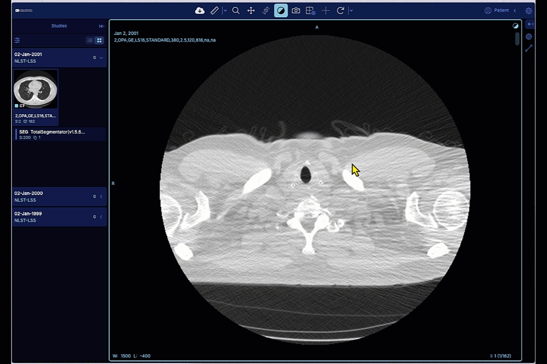
The version of the viewer is available from the "About" menu for the OHIF (radiology) viewer, and "Get app info" menu for the Slim (pathology) viewers. Both of those menus are in the upper right corner of the window.
IDC viewers release notes are maintained via GitHub Releases. Once you identified the version of the deployed viewer using the instructions above, you can locate the corresponding release notes in the following:
OHIF v3 release notes:
Slim release notes:
a significant portion of functionality available in Slim is implemented in the dicom-microscopy-viewer package, its releases are available here:
The final OHIF v2 published version is 4.12.45. Upstream changes based on v2 will be accessible through the v2-legacy branch (will not be published to NPM).
Main highlights from v2-legacy since 4.12.45:
Fix high and critical dependency issues reported by dependabot
Update SEG tolerance popup and update SEG thumbnail warning: Jump to first segment item image and show warning message only once on onChange events
Update to issues and PR templates
Address segmentation visibility toggle applied to all segmentations instead of the active one only
The OHIF Viewer is a zero-footprint medical image viewer provided by the . It is a configurable and extensible progressive web application with out-of-the-box support for image archives which support .
Main highlights of this release include:
Handle missing ReferencedInstanceSequence attribute: Update parsing logic to consider attribute as optional.
The OHIF Viewer is a zero-footprint medical image viewer provided by the . It is a configurable and extensible progressive web application with out-of-the-box support for image archives which support .
Main highlights of this release include:
Remove unused code from DICOM SR parsing: Remove referecenedImages attribute from SR display sets. Within TID 1500, sub-template TID 1600 (Image Library) is not required while parsing SR for image references for annotations and planar measurements. The same is obtained from sub template TID 1501>TID 300>TID 320.
The OHIF Viewer is a zero-footprint medical image viewer provided by the . It is a configurable and extensible progressive web application with out-of-the-box support for image archives which support .
Main highlights of this release include:
Update message for segmentation error loading due to orientation tolerance
The OHIF Viewer is a zero-footprint medical image viewer provided by the . It is a configurable and extensible progressive web application with out-of-the-box support for image archives which support .
Main highlights of this release include:
Correct Parsing Logic for Qualitative Instance Level SR
The OHIF Viewer is a zero-footprint medical image viewer provided by the . It is a configurable and extensible progressive web application with out-of-the-box support for image archives which support .
Main highlights of this release include:
Fix 2d MPR rendering issue for the sagittal view
Slim is a lightweight server-less single-page application for interactive visualization of digital slide microscopy (SM) images and associated image annotations in standard DICOM format. The application is based on the library and can simply be placed in front of a compatible Image Management System (IMS), Picture Archiving and Communication (PACS), or Vendor Neutral Archive (VNA).
New Features
Support configuration of multiple origin servers for different types of DICOM objects (SOP Storage Classes)
Enhancements
Improved error handling
Check Pyramid UID (if available) when grouping images into digital slides
Bug Fixes
Use Acquisition UID (if available) to group images into digital slides
The Slim Viewer is a lightweight server-less single-page application for interactive visualization of digital slide microscopy (SM) images and associated image annotations in standard DICOM format. The application is based on the library and can simply be placed in front of a compatible Image Management System (IMS), Picture Archiving and Communication (PACS), or Vendor Neutral Archive (VNA).
Main highlights of this release include:
New features
Add new tool to go to specific slide position;
Show mouse position in slide coordinate system.
Enhancements
Improve performance of translations between image and slide coordinates;
Automatically adjust size of overview image to size of browser window.
Bug fixes
Fix rendering of label image;
Show error message when creation of viewer fails;
Fix resolution of overview image;
Fix styling of point annotations;
The OHIF Viewer is a zero-footprint medical image viewer provided by the . It is a configurable and extensible progressive web application with out-of-the-box support for image archives which support .
Main highlights of this release include:
Fix parsing of qualitative slice annotation;
Disable measurements panel interactions in MPR mode;
Fix parsing of segmentation when orientation values are close to zero;
Raise error if a frame StudyInstanceUID, SeriesInstanceUID and SOPInstanceUID are not conforming with the UID (DICOM UI VR) character repertoire;
The Slim Viewer is a lightweight server-less single-page application for interactive visualization of digital slide microscopy (SM) images and associated image annotations in standard DICOM format. The application is based on the library and can simply be placed in front of a compatible Image Management System (IMS), Picture Archiving and Communication (PACS), or Vendor Neutral Archive (VNA).
Main highlights of this release include:
New features
Add panel for clinical trial information to case viewer;
Sort digital slides by Container Identifier attribute.
Enhancements
Reset style of optical paths to default when deactivating presentation state.
Bug fixes
Fix rendering of ROI annotations by upgrading to React version 1;
Correctly update UIDs of visible/active optical paths;
Fix type declarations of DICOMweb search resources.
The OHIF Viewer is a zero-footprint medical image viewer provided by the . It is a configurable and extensible progressive web application with out-of-the-box support for image archives which support .
Main highlights of this release include:
Add support for SR qualitative annotation per instance.
The Slim Viewer is a lightweight server-less single-page application for interactive visualization of digital slide microscopy (SM) images and associated image annotations in standard DICOM format. The application is based on the library and can simply be placed in front of a compatible Image Management System (IMS), Picture Archiving and Communication (PACS), or Vendor Neutral Archive (VNA).
Main highlights of this release include:
New features
Support DICOM Advanced Blending Presentation State to parametrize the display of multiplexed IF microscopy images;
Add key bindings for annotations tools;
Enable configuration of tile preload;
Enable configuration of annotation geometry type per finding;
Enhancements
Improve default presentation of multiplexed IF microscopy images in the absence of presentation state instances;
Correctly configure DCM4CHEE Archive to use reverse proxy URL prefix for BulkDataURI in served metadata;
Enlarge display settings interfaces and add input fields for opacity, VOI limits, and colors;
Update dicom-microscopy-viewer version to use web workers for frame decoding/transformation operations;
Bug fixes
Fix parsing of URL path upon redirect after successful authentication/authorization;
Fix configuration of optical path display settings when switching between presentation states;
Fix caching of presentation states and for selection via drop-down menu.
Security
Update dependencies with critical security issues.
The Slim Viewer is a lightweight server-less single-page application for interactive visualization of digital slide microscopy (SM) images and associated image annotations in standard DICOM format. The application is based on the library and can simply be placed in front of a compatible Image Management System (IMS), Picture Archiving and Communication (PACS), or Vendor Neutral Archive (VNA).
Main highlights of this release include:
Enhancements
Make overview panel collapsible and hide it entirely if lowest-resolution image is too large.
Bug fixes
Fix update of optical path settings when switching between slides.
The OHIF Viewer is a zero-footprint medical image viewer provided by the . It is a configurable and extensible progressive web application with out-of-the-box support for image archives which support .
Main highlights of this release include:
Fix regression in logic for finding segmentations referenced source image;
Fix segmentations loading issues;
Fix thumbnail series type for unsupported SOPClassUID;
Fix toolbar error when getDerivedDatasets finds no referenced series are found.
The Slim Viewer is a lightweight server-less single-page application for interactive visualization of digital slide microscopy (SM) images and associated image annotations in standard DICOM format. The application is based on the library and can simply be placed in front of a compatible Image Management System (IMS), Picture Archiving and Communication (PACS), or Vendor Neutral Archive (VNA).
Main highlights of this release include:
New features
Display of analysis results stored as DICOM Segmentation, Parametric Map, or Microscopy Bulk Simple Annotations instances;
Dynamic selection of DICOMweb server by user (can be enabled by setting AppConfig.enableServerSelection to true);
Dark app mode for fluorescence microscopy (can be enabled by setting App.mode to "dark");
Improvements
Unify handling of optical paths for color and grayscale images;
Add loading indicator;
Improve styling of overview map;
Render specimen metadata in compacter form;
Bug fixes
Ensure ROI annotations are re-rendered upon modification;
Clean up memory and recreate viewers upon page reload;
Fix selection of volume images;
Fix color space conversion during decoding of JPEG 2000 compressed image frames;
The OHIF Viewer is a zero-footprint medical image viewer provided by the . It is a configurable and extensible progressive web application with out-of-the-box support for image archives which support .
Main highlights of this release include:
Improve logic for finding segmentations referenced source image;
Improve debug dialog: fix text overflow and adding active viewports referenced SEGs and RTSTRUCT series.
The OHIF Viewer is a zero-footprint medical image viewer provided by the . It is a configurable and extensible progressive web application with out-of-the-box support for image archives which support .
Main highlights of this release include:
Fix fail to load SEG related to geometry assumptions;
Fix fail to load SEG related to tolerance;
Add initial support for SR planar annotations.
The Slim Viewer is a lightweight server-less single-page application for interactive visualization of digital slide microscopy (SM) images and associated image annotations in standard DICOM format. The application is based on the library and can simply be placed in front of a compatible Image Management System (IMS), Picture Archiving and Communication (PACS), or Vendor Neutral Archive (VNA).
Main highlights of this release include:
Bug fixes
Fix selection of VOLUME or THUMBNAIL images with different Photometric Interpretation.
The OHIF Viewer is a zero-footprint medical image viewer provided by the . It is a configurable and extensible progressive web application with out-of-the-box support for image archives which support .
Main highlights of this release include:
Fix RTSTRUCT right panel updates;
Fix SEG loading regression.
The OHIF Viewer is a zero-footprint medical image viewer provided by the . It is a configurable and extensible progressive web application with out-of-the-box support for image archives which support .
Main highlights of this release include:
Fix handling of datasets with unsupported modalities;
Fix backward fetch of images for the current active series.
Fix tag browser slider.
The Slim Viewer is a lightweight server-less single-page application for interactive visualization of digital slide microscopy (SM) images and associated image annotations in standard DICOM format. The application is based on the library and can simply be placed in front of a compatible Image Management System (IMS), Picture Archiving and Communication (PACS), or Vendor Neutral Archive (VNA).
Main highlights of this release include:
Bug fixes
Rotate box in overview map outlining the extent of the current view together with the image.
The OHIF Viewer is a zero-footprint medical image viewer provided by the . It is a configurable and extensible progressive web application with out-of-the-box support for image archives which support .
Main highlights of this release include:
Fix segmentation/rtstruct menu badge update when switching current displayed series;
Add to series thumbnail link icon if they are connected to any annotation (segmentation, etc...);
Fix problems opening series when the study includes many series;
Fix segments visibility handler.
The Slim Viewer is a lightweight server-less single-page application for interactive visualization of digital slide microscopy (SM) images and associated image annotations in standard DICOM format. The application is based on the library and can simply be placed in front of a compatible Image Management System (IMS), Picture Archiving and Communication (PACS), or Vendor Neutral Archive (VNA).
Main highlights of this release include:
Improvements
Include images with new flavor THUMBNAIL in image pyramid;
Properly fit overview map into HTML element and disable re-centering of overview map when user navigates main map;
Allow drawing of ROIs that extent beyond the slide coordinate system (i.e., allow negative ROI coordinates).
Bug fixes
Prevent display of annotation marker when ROI is deactivated
The OHIF Viewer is a zero-footprint medical image viewer provided by the . It is a configurable and extensible progressive web application with out-of-the-box support for image archives which support .
Main highlights of this release include:
Fix issues with segmentation orientations;
Fix display of inconsistencies warning for segmentation thumbnails;
Fix throttle thumbnail progress updates.
The Slim Viewer is a lightweight server-less single-page application for interactive visualization of digital slide microscopy (SM) images and associated image annotations in standard DICOM format. The application is based on the library and can simply be placed in front of a compatible Image Management System (IMS), Picture Archiving and Communication (PACS), or Vendor Neutral Archive (VNA).
Main highlights of this release include:
Bug fixes
Set PUBLIC_URL in Dockerfile.
The Slim Viewer is a lightweight server-less single-page application for interactive visualization of digital slide microscopy (SM) images and associated image annotations in standard DICOM format. The application is based on the library and can simply be placed in front of a compatible Image Management System (IMS), Picture Archiving and Communication (PACS), or Vendor Neutral Archive (VNA).
Main highlights of this release include:
Improvements
Add button to display information about application and environment;
Add ability to include logo;
Verify content of SR documents before attempting to load annotations;
Improve re-direction after authentication;
Bug fixes
Disable zoom of overview map;
Fix pagination of worklist;
Prevent delay in tile rendering.
The OHIF Viewer is a zero-footprint medical image viewer provided by the . It is a configurable and extensible progressive web application with out-of-the-box support for image archives which support .
Main highlights of this release include:
Handle uncaught exception for non TID 1500 sr;
Added display of badge numbers in the segmentation / rtstruct panel tabs;
Study prefetcher with loading bar.
The Slim Viewer is a lightweight server-less single-page application for interactive visualization of digital slide microscopy (SM) images and associated image annotations in standard DICOM format. The application is based on the library and can simply be placed in front of a compatible Image Management System (IMS), Picture Archiving and Communication (PACS), or Vendor Neutral Archive (VNA).
Main highlights of this release include:
New features
Support for multiplexed immunofluorescence slide microscopy imaging;
Client-side additive blending of multiple channels using WebGL;
Client-side decoding of compressed frame items using WebAssembly based on Emscripten ports of libjpeg-turbo, openjpeg, and charls C/C++ libraries.
Improvements
Continuous integration testing pipeline using circle CI;
Deploy previews for manual regression testing.
Major changes
Introduce new configuration parameter renderer.
The OHIF Viewer is a zero-footprint medical image viewer provided by the . It is a configurable and extensible progressive web application with out-of-the-box support for image archives which support .
Main highlights of this release include:
Add exponential backoff and retry after 500 error;
Update to HTML SR viewport to display missing header tags.
The Slim Viewer is a lightweight server-less single-page application for interactive visualization of digital slide microscopy (SM) images and associated image annotations in standard DICOM format. The application is based on the library and can simply be placed in front of a compatible Image Management System (IMS), Picture Archiving and Communication (PACS), or Vendor Neutral Archive (VNA).
Inital Release.
The OHIF Viewer is a zero-footprint medical image viewer provided by the . It is a configurable and extensible progressive web application with out-of-the-box support for image archives which support .
Main highlights of this release include:
Add disable server cache feature;
Additional improvements on series inconsistencies report UI.
The OHIF Viewer is a zero-footprint medical image viewer provided by the . It is a configurable and extensible progressive web application with out-of-the-box support for image archives which support .
Main highlights of this release include:
Add acquisition storage SR sopclass to SR html ext;
Fix missing items in the segmentation combobox items at loading;
Fix slices are not sorted in geometrical order;
Extend series inconsistencies checks to segmentation and improve UI.
The OHIF Viewer is a zero-footprint medical image viewer provided by the . It is a configurable and extensible progressive web application with out-of-the-box support for image archives which support .
Main highlights of this release include:
Add new log service to be used by debugger extension;
Add UI to communicate to the users inconsistencies within a single series;
Add time in the dates of the items of the segmentation combobox list;
Order segmentation combobox list in reverse time order;
The OHIF Viewer is a zero-footprint medical image viewer provided by the . It is a configurable and extensible progressive web application with out-of-the-box support for image archives which support .
Main highlights of this release include:
Replace instance dropdown to slider for dicom tag browser;
Add error page and not found pages if failed to retrieve study data.
The OHIF Viewer is a zero-footprint medical image viewer provided by the . It is a configurable and extensible progressive web application with out-of-the-box support for image archives which support .
Main highlights of this release include:
Add UI error report for MPR buffer limit related errors;
Add UI error report for hardware acceleration turned off errors;
Add IDC funding acknowledgment;
Fix RSTRUCT menu panel undefined variables;
The OHIF Viewer is a zero-footprint medical image viewer provided by the . It is a configurable and extensible progressive web application with out-of-the-box support for image archives which support .
Main highlights of this release include:
Visualize overlapping segments;
Use runtime value configuration to get pkg version;
Fix navigation issues in the crosshair tool.
The OHIF Viewer is a zero-footprint medical image viewer provided by the . It is a configurable and extensible progressive web application with out-of-the-box support for image archives which support .
Main highlights of this release include:
Add MPR crosshair tool.
Update dcmjs version so it throws 'Failed to find the reference image in the source data. Cannot load this segmentation' error instead of logging a warning to console
Address eye icon for segment not shown when segment name is long
Change message for segmentation when it fails to load duo to orientation tolerance
Ensure bounding box annotations are axis aligned;
Add missing keyboard shortcut for navigation tool.
Implements runtime tolerance for SEGs loading retry;
Fixed popup notifications behavior;
Update cornerstoneWADOImageLoader.
Expose equipment metadata in user interface.
Add button for user logout;
Disable optical path selection when a presentation state has been selected.
Support display of parameter mappings stored in DICOM Parametric Map instances;
Support display of annotation groups stored in DICOM Microscopy Bulk Simple Annotations instances;
Implement color transformations using ICC Profiles to correct color images client side in a browser-independent manner;
Implement grayscale transformations using Palette Color Lookup Tables to pseudo-color grayscale images.
Improve fetching of WASM library code;
Improve styling of slide viewer sidebar;
Sort slides by Series Number;
Work around common standard compliance issues;
Update docker-compose configuration;
Upgrade dependencies;
Show examples in README;
Decode JPEG, JPEG 2000, and JPEG-LS compressed image frames client side in a browser-independent manner;
Improve performance of transformation and rendering operations using WebGL for both grayscale as well as color images;
Optimize display of overview images and keep overview image fixed when zooming or panning volume images;
Optimize HTTP Accept header field for retrieval of frames to work around issues with various server implementations.
Fix unit of area measurements for ROI annotations;
Publish events when bulkdata loading starts and ends.
Add retry logic and error handlers for DICOMweb requests;
Improve documentation of application configuration in README;
Add unit tests.
Fix failure to load a valid SEG object because of incorrect expectations about ReferencedSegmentNumber;
Fix RSTRUCT menu visibility when loading a series;
Fix image load slowness regression;
Fix choppy scrolling in 2D mod;
Fix failure to load segmentations when filtering study with '?seriesInstanceUID=' syntax.
Fix RSTRUCT menu visibility when loading a series;
Fix segments visibility control (SEG menu) bugs .


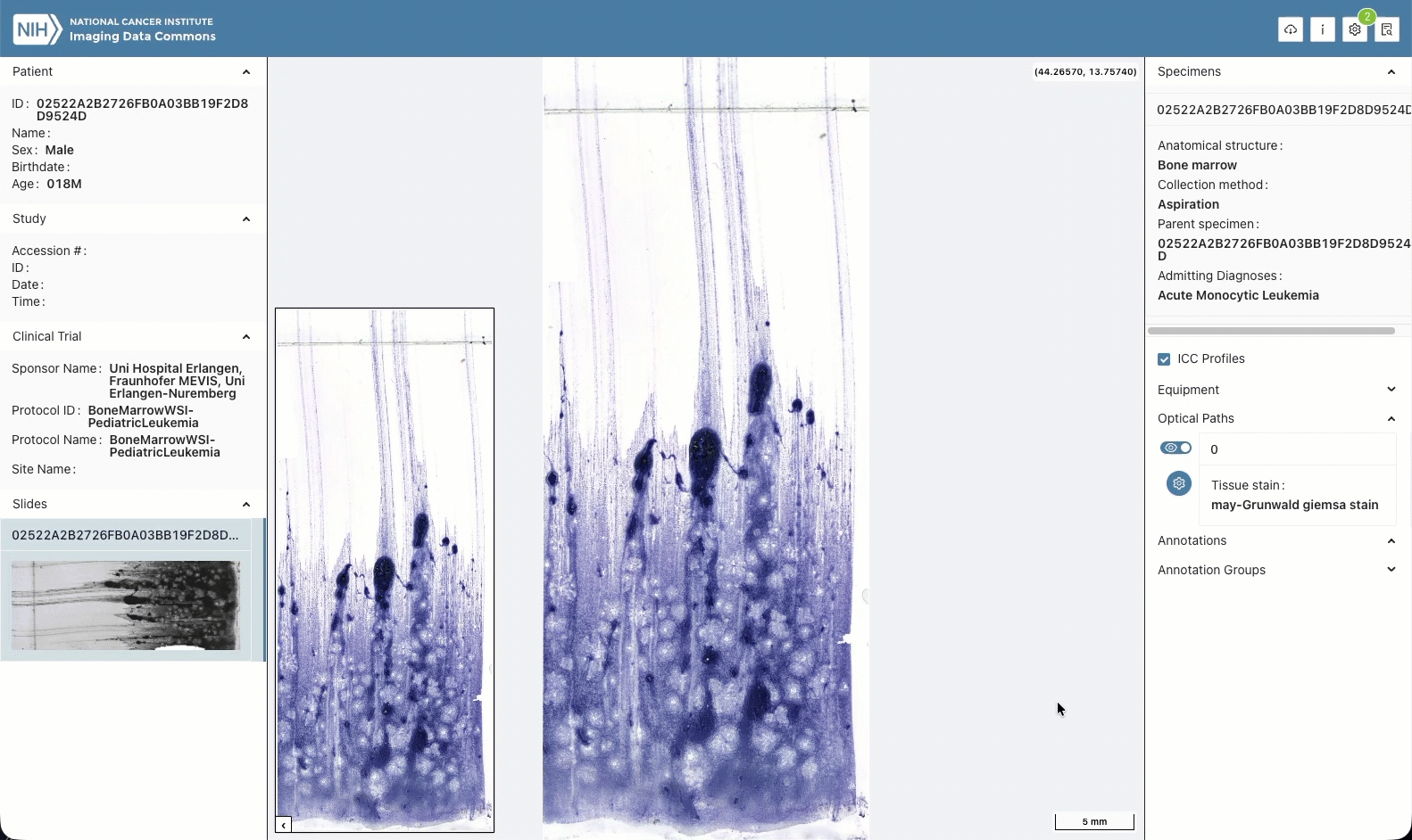
A manifest is a table of access methods and other metadata of the objects in some cohort. The POST /cohorts/manifest/preview API endpoint
The POST /cohorts/manifest/preview API accepts both a fields list, and a cohort definition in the manifestPreviewBody, and returns a manifest. The JSON schema of the manifestBody can be seen on the IDC API v2 UI page. Here is an example:
As previously mentioned, it behaves as if a cohort is created, a manifest for that cohort is returned and the new cohort is deleted.
The filters parameter specifies a filter set that defines the cohort.
The fields parameter of the body indicates the fields whose values are to be included in the returned manifests. The /fields API endpoint returns a list of the fields that can be included in a manifest.
The counts, group_size, sql and page_size parameters will be described in subsequent sections.
Every row in the returned manifest will include one value for each of the items in the fields parameter.
The /cohorts/manifest/preview returns a manifestPreviewResponse JSON object. Here is an example manifestResponse:
The cohort definition is included so that the manifest is self-documenting. The manifest_data component of the manifest component contains a row for each distinct combination of the requested fields in the cohort.
Because the /cohorts/manifest/preview API endpoint is always applied against the current IDC version, the idc_data_version in the cohort_def is always that of the current IDC version. This version information can be useful if the cohort_def is saved.
The totalFound value at the end of the manifest tells us that there are 626 rows in the manifest, meaning the manifest contains 626 different combinations of Modality, SliceThickness, age_at_diagnosis, aws_bucket, and crdc_series uuid.
The rowsReturned value indicates that all the rows in the manifest were return in the first "page". If not all the rows had been returned, we can ask for additional "pages" as described in the next section.
The next_page value is described in the next section.
We use the term group to indicate the set of all instances in the cohort having the values of some row in the manifest. Thus the values of the first row above:
implicitly define a group of instances in the cohort, each of which has those values.
When the group_size parameter in the manifestPreviewBody is true, the resulting manifest includes the total size in bytes of the instances in the corresponding group. Following is a fragment of the manifest for the same cohort above, but where the fields list has "group_size": true:
Here we see that the instances in the group corresponding to the first result row have a total size of 2,690,320B.
The group_size parameter is optional and defaults to false .
If the counts parameter is true, the resulting manifest will selectively include counts of the instances, series, studies, patients and collections in each group. Which counts are included in a manifest is determined by the granularity, and which, in turn, is determined by certain of the possible fields in the fields parameter list of the manifestPreviewBody.
For example, if the fields parameter list includes the SOPInstanceUID field, there will one group per instance in the manifest. Thus the manifest has instance granularity. A manifest has just one of instance, series, study, patient, collection or version granularity.
For a given manifest granularity, and when counts is True, counts of the "lower level" objects are reported in the manifest. Thus, if a cohort has series granularity, then the count of all instances in each group is reported. If a cohort has study granularity, then the count of all instances in each group and of all series in each group are reported. And so on. This is described in detail in the remainder of this section.
In the following, manifest examples are based on this filterSet:
A manifest will have instance granularity if the fields parameter list includes one or both of the fields:
SOPInstanceUID
crdc_instance_uuid
gcs_url
aws_url
Both of these fields are unique to each instance. Therefore the resulting manifest will include one row for each instance in the specified cohort. For example, the following fields list will result in a manifest having a row per instance:
Each row will include the SOPInstanceUID, and the Modality and SliceThickness of the corresponding instance.
The counts parameter is ignored because there are no 'lower level' objects than instances in the DICOM hierarchy.
A manifest will have series granularity if it does not have instance granularity and the fields parameter list includes one or more of thee field:
SeriesInstanceUID
crdc_series_uuid
Both of these fields are unique to each series, and therefore the resulting manifest will include at least one row per series in the specified cohort. For example, the following fields list will result in a manifest having one or more rows per series:
Because the SeriesInstanceUID is unique to each series in a cohort (more accurately, all instances in a series have the same SeriesInstanceUID), there will be at least one row per series in the resulting manifest. However, SliceThickness is not necessarily unique across all instance in a series. Therefore, the resulting manifest may have multiple rows for a given series...rows in which the SeriesInstanceUID is the same but the SliceThickness values differ. DICOM modality should always be the same for all instances in a series; therefore it is not expected to result in multiple rows per series.
If the counts parameter is true, each row of the manifest will have:
an instance_count value that is the count of instances in the group corresponding to the row
Given the above fields, then this is a fragment of the series granularity manifest of our example cohort:
This tells us that the group of instances corresponding to the first row of the manifest results has 151 members.
A manifest will have study granularity if it does not have series or instance granularity and the queryFields list includes one or more of the fields:
StudyInstanceUID
crdc_study_uuid
Both of these fields are unique to each study, and therefore the resulting manifest will include at least one row per study in the specified cohort. For example, the following fields list will result in a manifest having a one or more rows per study:
SliceThickness can vary not only among the instances in a series, but among series in a study. Therefore, the resulting manifest may have multiple rows for a study, and which differ from each other in both SliceThickness and Modality.
If counts is in the fields list, each row of the manifest will have:
an instance_count value that is the count of instances in the group corresponding to the row
a series_count value that is the count of series in the group corresponding to the row
If the fields list is as above, then this is a fragment of the study granularity manifest of our example cohort:
This tells us that the group of instances corresponding to the first row of the manifest results has 212 members, divided among two series. The group of instances corresponding to the third row of the manifest results has two members in a single series.
A manifest will have patient granularity if it goes not have study, series or instance granularity and the fields list includes the field PatientID. This field is unique to each patient, and therefore the resulting manifest will include at least one row per patient in the specified cohort. For example, the following fields list will result in a manifest having a one or more rows per study:
Because the PatientID is unique to each patient in a cohort (more accurately, all instances in a study have the same PatientID), there will be at least one row per patient in the resulting manifest. It is common for a patient's series to examine different body parts. Therefore, the resulting manifest may well have more than one row per patient.
If counts is in the fields list, each row of the manifest will have:
an instance_count value that is the count of instances in the group corresponding to the row
a series_count value that is the count of series in the group corresponding to the row
a study_count value that is the count of studies in the group corresponding to the row
If the fields list is as above, then this is a fragment of the patient granularity manifest of our example cohort:
This tells us that the group of instances corresponding to the first row of the manifest results has 212 members divided among two series, and both in a single study.
A manifest will have collection granularity if it goes not have patient, study, series or instance granularity and the fields parameter list includes the field collection_id. This field is unique to each collection, and therefore the resulting manifest will include at least one row per collection in the specified cohort. For example, the following fields list will result in a manifest having a one or more rows per study:
Because the collection_id is unique to each collection in a cohort (more accurately, all instances in a collection have the same collection_id), there will be at least one row per collection in the resulting manifest. It is common for a collection to have patients of different ages. Therefore, the resulting manifest may well have more than one row per patient.
If the fields list is as above, then this is a fragment of the collection granularity manifest of our example cohort:
A manifest will have version granularity if it does not have collection, patient, study, series or instance granularity. At this granularity level, the rows in the manifest return the combinations of queried values across all collects, patients, studies, series and instances in the cohort.
When the fields list is as follows:
then this is a fragment of the version granularity manifest of our example cohort:
Row one of the results tells us that the cohort has 212 instances having a Null SliceThickness and modality="CT". Also, there are apparently 87 different combinations of Modality and SliceThickness in the cohort as shown by the totalFound value.
{
"cohort_def": {
"name": "mycohort",
"description": "Example description",
"filters": {
"collection_id": [
"TCGA_luad",
"%_kirc"
],
"Modality": [
"CT",
"MR"
],
"Race": [
"WHITE"
],
"age_at_diagnosis_btw": [
65,
75
]
}
},
"fields": [
"Age_At_Diagnosis",
"aws_bucket",
"crdc_series_uuid",
"Modality",
"SliceThickness"
],
"counts": true,
"group_size": true,
"sql": true,
"page_size": 1000
}
{
"code": 200,
"cohort_def": {
"description": "Example description",
"user_email": "[email protected]",
"filterSet": {
"filters": {
"Modality": [
"CT",
"MR"
],
"age_at_diagnosis_btw": [
65,
75
],
"collection_id": [
"tcga_luad",
"%_kirc"
],
"race": [
"WHITE"
]
},
"idc_data_version": "16.0"
},
"name": "mycohort",
},
"manifest": {
"manifest_data": [
{
"Modality": "MR",
"SliceThickness": "10.0",
"age_at_diagnosis": 66,
"aws_bucket": "idc-open-data",
"crdc_series_uuid": "09bc812b-53f7-48fc-8895-72f6b03f642b"
},
{
"Modality": "CT",
"SliceThickness": "2.5",
"age_at_diagnosis": 66,
"aws_bucket": "idc-open-data",
"crdc_series_uuid": "102d676d-6c6f-4c20-bb36-77ec81b81b13"
},
{
"Modality": "CT",
"SliceThickness": "8.0",
"age_at_diagnosis": 66,
"aws_bucket": "idc-open-data",
"crdc_series_uuid": "1d365f52-bff4-4348-a508-82d399ca8442"
},
:
{
"Modality": "CT",
"SliceThickness": "1000.090881",
"age_at_diagnosis": 74,
"aws_bucket": "idc-open-data",
"crdc_series_uuid": "faa47e10-45df-44a7-9f8b-2923a41196b4"
}
],
"rowsReturned": 626,
"totalFound": 626
},
"next_page": ""
}
"Modality": "MR",
"SliceThickness": "10.0",
"age_at_diagnosis": 66,
"aws_bucket": "idc-open-data",
"crdc_series_uuid": "09bc812b-53f7-48fc-8895-72f6b03f642b" {
"code": 200,
"cohort_def": {
"description": "Example description",
"filterSet": {
"filters": {
"Modality": [
"CT",
"MR"
],
"age_at_diagnosis_btw": [
65,
75
],
"collection_id": [
"tcga_luad",
"tcga_kirc"
],
"race": [
"WHITE"
]
},
"idc_data_version": "16.0"
},
"name": "mycohort",
"sql": ""
},
"next_page": "",
"manifest": {
"manifest_data": [
{
"Modality": "MR",
"SliceThickness": "10.0",
"age_at_diagnosis": 66,
"aws_bucket": "idc-open-data",
"crdc_series_uuid": "09bc812b-53f7-48fc-8895-72f6b03f642b",
"group_size": 2690320
},
{
"Modality": "CT",
"SliceThickness": "2.5",
"age_at_diagnosis": 66,
"aws_bucket": "idc-open-data",
"crdc_series_uuid": "102d676d-6c6f-4c20-bb36-77ec81b81b13",
"group_size": 42818868
},
{
"Modality": "CT",
"SliceThickness": "8.0",
"age_at_diagnosis": 66,
"aws_bucket": "idc-open-data",
"crdc_series_uuid": "1d365f52-bff4-4348-a508-82d399ca8442",
"group_size": 20064536
},
:
:
{
"Modality": "CT",
"SliceThickness": "1000.090881",
"age_at_diagnosis": 74,
"aws_bucket": "idc-open-data",
"crdc_series_uuid": "faa47e10-45df-44a7-9f8b-2923a41196b4",
"group_size": 6518724
}
],
"rowsReturned": 626,
"totalFound": 626
},
"next_page": ""
} "filters": {
"collection_id": [
"tcga_luad",
"tcga_kirc"
],
"Modality": [
"CT",
"MR"
],
"Race": [
"WHITE"
],
"age_at_diagnosis_btw": [
65,
75
]
}
{
"fields": [
"SOPInstanceUID",
"Modality",
"SliceThickness"
]
}"fields": [
"Modality",
"SliceThickness",
"collection_id",
"patientID",
"StudyInstanceUID",
"SeriesInstanceUID"
]{
"code": 200,
"cohort_def": {
"description": "Example description",
"filterSet": {
"filters": {
"Modality": [
"CT",
"MR"
],
"age_at_diagnosis_btw": [
65,
75
],
"collection_id": [
"tcga_luad",
"tcga_kirc"
],
"race": [
"WHITE"
]
},
"idc_data_version": "16.0"
},
"name": "mycohort",
"sql": ""
},
"manifest": {
"manifest_data": [
{
"Modality": "CT",
"PatientID": "TCGA-50-6592",
"SeriesInstanceUID": "1.3.6.1.4.1.14519.5.2.1.6450.9002.141004994853145237754973938025",
"SliceThickness": null,
"StudyInstanceUID": "1.3.6.1.4.1.14519.5.2.1.6450.9002.256822832756566055874151999412",
"collection_id": "tcga_luad",
"instance_count": "151"
},
{
"Modality": "CT",
"PatientID": "TCGA-50-6592",
"SeriesInstanceUID": "1.3.6.1.4.1.14519.5.2.1.6450.9002.212096199865546132848990878032",
"SliceThickness": null,
"StudyInstanceUID": "1.3.6.1.4.1.14519.5.2.1.6450.9002.256822832756566055874151999412",
"collection_id": "tcga_luad",
"instance_count": "61"
},
{
"Modality": "CT",
"PatientID": "TCGA-50-6595",
"SeriesInstanceUID": "1.3.6.1.4.1.14519.5.2.1.6450.9002.829269157955398706933292266867",
"SliceThickness": "0.578125",
"StudyInstanceUID": "1.3.6.1.4.1.14519.5.2.1.6450.9002.414530650520592976265083061155",
"collection_id": "tcga_luad",
"instance_count": "1"
},
:
:
{
"Modality": "MR",
"PatientID": "TCGA-B0-5109",
"SeriesInstanceUID": "1.3.6.1.4.1.14519.5.2.1.6450.4004.370888372270096165934432087127",
"SliceThickness": "20.0",
"StudyInstanceUID": "1.3.6.1.4.1.14519.5.2.1.6450.4004.167173047835125001355984228239",
"collection_id": "tcga_kirc",
"instance_count": "50"
}
],
"rowsReturned": 742,
"totalFound": 742
}
"next_page": ""
}"fields": [
"Modality",
"SliceThickness",
"collection_id",
"patientID",
"StudyInstanceUID",
"group_size",
"counts"
]{
"code": 200,
"cohort_def": {
"description": "Example description",
"filterSet": {
"filters": {
"Modality": [
"CT",
"MR"
],
"age_at_diagnosis_btw": [
65,
75
],
"collection_id": [
"tcga_luad",
"tcga_kirc"
],
"race": [
"WHITE"
]
},
"idc_data_version": "16.0"
},
"name": "mycohort",
"sql": ""
},
"manifest": {
"manifest_data": [
{
"Modality": "CT",
"PatientID": "TCGA-50-6592",
"SliceThickness": null,
"StudyInstanceUID": "1.3.6.1.4.1.14519.5.2.1.6450.9002.256822832756566055874151999412",
"collection_id": "tcga_luad",
"instance_count": 212,
"series_count": 2
},
{
"Modality": "CT",
"PatientID": "TCGA-50-6595",
"SliceThickness": "0.578125",
"StudyInstanceUID": "1.3.6.1.4.1.14519.5.2.1.6450.9002.414530650520592976265083061155",
"collection_id": "tcga_luad",
"instance_count": 1,
"series_count": 1
},
{
"Modality": "CT",
"PatientID": "TCGA-B8-4153",
"SliceThickness": "0.6",
"StudyInstanceUID": "1.3.6.1.4.1.14519.5.2.1.8421.4004.499780439902438461273732269226",
"collection_id": "tcga_kirc",
"instance_count": 2,
"series_count": 1
},
:
:
{
"Modality": "MR",
"PatientID": "TCGA-B0-5109",
"SliceThickness": "20.0",
"StudyInstanceUID": "1.3.6.1.4.1.14519.5.2.1.6450.4004.167173047835125001355984228239",
"collection_id": "tcga_kirc",
"instance_count": 100,
"series_count": 2
}
],
"rowsReturned": 324,
"totalFound": 324
},
"next_page": ""
}"fields": [
"Modality",
"SliceThickness",
"collection_id",
"patientID",
"group_size",
"counts"
]{
"code": 200,
"cohort_def": {
"description": "Example description",
"filterSet": {
"filters": {
"Modality": [
"CT",
"MR"
],
"age_at_diagnosis_btw": [
65,
75
],
"collection_id": [
"tcga_luad",
"tcga_kirc"
],
"race": [
"WHITE"
]
},
"idc_data_version": "16.0"
},
"name": "mycohort",
"sql": ""
},
"next_page": "",
"manifest": {
"manifest_data": [
{
"Modality": "CT",
"PatientID": "TCGA-50-6592",
"SliceThickness": null,
"collection_id": "tcga_luad",
"instance_count": "212",
"series_count": "2",
"study_count": "1"
},
{
"Modality": "CT",
"PatientID": "TCGA-50-6595",
"SliceThickness": "0.578125",
"collection_id": "tcga_luad",
"instance_count": "1",
"series_count": "1",
"study_count": "1"
},
{
"Modality": "CT",
"PatientID": "TCGA-B8-4153",
"SliceThickness": "0.6",
"collection_id": "tcga_kirc",
"instance_count": "6",
"series_count": "2",
"study_count": "2"
},
:
:
{
"Modality": "MR",
"PatientID": "TCGA-B0-5109",
"SliceThickness": "20.0",
"collection_id": "tcga_kirc",
"instance_count": "100",
"series_count": "2",
"study_count": "1"
}
],
"rowsReturned": 301,
"totalFound": 301
}
}"fields": [
"Modality",
"SliceThickness",
"collection_id",
"patientID",
"group_size",
"counts"
]{
"code": 200,
"cohort_def": {
"description": "Example description",
"filterSet": {
"filters": {
"Modality": [
"CT",
"MR"
],
"age_at_diagnosis_btw": [
65,
75
],
"collection_id": [
"tcga_luad",
"tcga_kirc"
],
"race": [
"WHITE"
]
},
"idc_data_version": "16.0"
},
"name": "mycohort",
"sql": ""
},
"manifest": {
"manifest_data": [
{
"Modality": "CT",
"SliceThickness": null,
"collection_id": "tcga_luad"
"instance_count": "212",
"patient_count": "1",
"series_count": "2",
"study_count": "1"
},
{
"Modality": "CT",
"SliceThickness": "0.578125",
"collection_id": "tcga_luad",
"instance_count": "1",
"patient_count": "1",
"series_count": "1",
"study_count": "1"
},
{
"Modality": "CT",
"SliceThickness": "0.6",
"collection_id": "tcga_kirc",
"instance_count": "29",
"patient_count": "9",
"series_count": "16",
"study_count": "14"
},
:
:
{
"Modality": "MR",
"SliceThickness": "20.0",
"collection_id": "tcga_kirc",
"instance_count": "100",
"patient_count": "1",
"series_count": "2",
"study_count": "1"
}
],
"rowsReturned": 88,
"totalFound": 88
}
"next_page": "",
}"fields": [
"Modality",
"SliceThickness",
"patientID",
"group_size",
"counts"
]{
"code": 200,
"cohort_def": {
"description": "Example description",
"filterSet": {
"filters": {
"Modality": [
"CT",
"MR"
],
"age_at_diagnosis_btw": [
65,
75
],
"collection_id": [
"tcga_luad",
"tcga_kirc"
],
"race": [
"WHITE"
]
},
"idc_data_version": "16.0"
},
"name": "mycohort",
"sql": ""
},
"manifest": {
"manifest_data": [
{
"Modality": "CT",
"SliceThickness": null,
"collection_count": "1",
"instance_count": "212",
"patient_count": "1",
"series_count": "2",
"study_count": "1"
},
{
"Modality": "CT",
"SliceThickness": "0.578125",
"collection_count": "1",
"instance_count": "1",
"patient_count": "1",
"series_count": "1",
"study_count": "1"
},
{
"Modality": "CT",
"SliceThickness": "0.6",
"collection_count": "2",
"instance_count": "34",
"patient_count": "11",
"series_count": "19",
"study_count": "17"
},
{
:
:
{
"Modality": "MR",
"SliceThickness": "20.0",
"collection_count": "1",
"instance_count": "100",
"patient_count": "1",
"series_count": "2",
"study_count": "1"
}
],
"rowsReturned": 87,
"totalFound": 87
}
"next_page": "",
}Release counts
Files: 46,870,903 (+175,736)
Series: 994,073 (+28,666)
Studies: 160,199 (+606)
Cases: 79,889 (+355)
Collections analyzed:
Lung-PET-CT-Dx
Collections analyzed:
NLST
varepop_apollo_clinical
Release counts
Files: 46,695,167 (+910,713)
Series: 965,407 (+14,519)
Studies: 159,593 (+10,016)
Cases: 79,214 (+8,132)
bonemarrowwsi_pediatricleukemia_clinical
cbis_ddsm_calc_case_description_test_set
cbis_ddsm_calc_case_description_train_set
cbis_ddsm_mass_case_description_test_set
varepop_apollo_clinical
bamf_aimi_annotations_brain_mr_qa_results
bamf_aimi_annotations_breast_fdg_pet_ct_qa_results
bamf_aimi_annotations_breast_mr_qa_results
bamf_aimi_annotations_kidney_ct_qa_results
nlst_canc
Previously nlst_clinical
acrin_nsclc_fdg_pet_bamf_lung_pet_ct_segmentation
Subsumed by bamf_aimi_annotations_lung_fdg_pet_ct_qa_results
anti_pd_1_lung_bamf_lung_ct_segmentation
Subsumed by bamf_aimi_annotations_lung_ct_qa_results
Collections analyzed:
Collections analyzed:
New pathology collections
New analysis results
Collections analyzed:
Collections analyzed:
Revised radiology collections
Cancer Moonshot Biobank (CMB) radiology images were updated to fix incorrect values assigned to PatientID (see details on the collection pages linked above). The updated images have different DICOM Study/Series/SOPInstanceUIDs.
Revised analysis results
Collections analyzed:
New clinical metadata tables
New radiology collections
New analysis results
* Collections analyzed:
** Collections analyzed:
Revised radiology collections
(starred collections are revised due to new or revised analysis results)
(revisions only to clinical data)
**
Revised pathology collections
(starred collections are revised due to new or revised analysis results)
(fix PatientAges > 090Y)
(fix PatientAges > 090Y)
*
Also added missing instance SOPInstanceUID: 1.3.6.1.4.1.5962.99.1.3459553143.523311062.1687086765943.9.0
New clinical metadata tables
Notes
The deprecated columns tcia_api_collection_id and idc_webapp_collection_id have been removed from the auxiliary_metadata table in the idc_v18 BQ dataset. These columns were duplicates of columns collection_name and collection_id respectively.
New radiology collections
New analysis results
Collections analyzed:
Revised radiology collections
New clinical metadata tables
New radiology collections
New pathology collections
Revised radiology collections
(TCIA description: (Repair of DICOM tag(0008,0005) to value "ISO_IR 100" in 79 series)
(Revised because results from CPTAC-CRCC-Tumor-Annotations were added)
(Revised because results from CPTAC-UCEC-Tumor-Annotations were added)
New analysis results
New clinical metadata tables
New radiology collections
New pathology collections
(ICDC-Glioma radiology added in a previous version)
Revised radiology collections
(TCIA description: “Radiology modality data cleanup to remove extraneous scans.”)
(“TCIA description: Radiology modality data cleanup to remove extraneous scans.”)
(TCIA description: “Radiology modality data cleanup to remove extraneous scans.”)
Revised pathology collections
(11 pathology-only patients removed at request of data owner)
(1 pathology-only patient removed at request of data owner)
New analysis results
(Analysis of NLST and NSCLC-Radiomics)
Revised analysis results
(Annotations of NLST and NSCLC-Radiomics radiology)
New clinical metadata tables
This release does not introduce any new data, but changes the bucket organization and introduces replication of IDC files in Amazon AWS storage buckets, as described in .
New analysis results collection:
New clinical data collections:
New collections:
Updated collections:
Other:
Metadata corresponding to "limited" access collections are removed.
New clinical data collections:
Other clinical data updates:
Limited access collections are removed. Clinical metadata for the COVID-19-NY-SUB and ACRIN 6698/I-SPY2 Breast DWI collections now includes information ingested from data dictionaries associated with these collections. In v11 the string value 'NA' was being changed to null during the ETL process for some columns/collections. This is now fixed in v12 and the value 'NA' is preserved.
This release introduces clinical data ingested for a subset of collections, and now available via a dedicated BigQuery dataset.
New collections:
In this release we introduce a new HTAN program including currently three collections release by the .
New collections:
Updated collections:
CPTAC, TCGA and NLST collections have been reconverted due to a technical issue identified with a subset of images included in v9.
*
Note that the TCGA-KIRP and TCGA-BRCA collections (marked with the asterisk in the list above) are currently missing SM high resolution layer files/instances due to a of Google Healthcare that makes it not possible to ingest datasets that exceed some internal limits. Specifically, the following patient/studies are affected:
TCGA-KIRP: PatientID TCGA-5P-A9KA, StudyInstanceUID 2.25.191236165605958868867890945341011875563
TCGA-BRCA: PatientID TCGA-OL-A66H, StudyInstanceUID 2.25.82800314486527687800038836287574075736 The affected files will be included in IDC when the infrastructure limitation is addressed.
Collection access level change:
is now available as public access collection
This data release introduces the concept of differential license to IDC: some of the collections maintained by IDC contain items that have different licenses. As an example, radiology component of the TCGA-GBM collection is covered by the TCIA limited access license, and is not available in IDC, while the digital pathology component is covered by CC-BY. With this release, we complete sharing in full of the digital pathology component of the datasets released by the CPTAC and TCGA programs.
New collections:
Updated collections:
The main highlight of this release is the addition of the NLST and TCGA Slide Microscopy imaging data. New TCGA content includes introduction of new (to IDC) TCGA collections that have only slide microscopy component, and addition of the slide microscopy component to those IDC collections that were available earlier and included only the radiology component.
New collections
TCGA-DLBC (TCGA-DLBC collection does not have a description page)
Updated collections
The main highlight of this release is the addition of the Slide Microscopy imaging component to the remaining CPTAC collections.
New collections
Updated collections
The following collections became limited access due to the , which is the original source of those collections.
Original collections:
Analysis results collections:
New collections:
New analysis results collections:
Outcome Prediction in Patients with Glioblastoma by Using Imaging, Clinical, and Genomic Biomarkers: Focus on the Nonenhancing Component of the Tumor ()
DICOM-SEG Conversions for TCGA-LGG and TCGA-GBM Segmentation Datasets ()
Updated collections:
is added. The data included consists of the following components:
1) CT images available as any other imaging collection (via IDC Portal, BigQuery metadata tables, and storage buckets);
2) a subset of clinical data available in the BigQuery tables starting with nlst_ under the idc_v4 dataset, as documented in the section.
3) One instance is missing from patient/study/series:
126153/1.2.840.113654.2.55.319335498043274792486636919135185299851/1.2.840.113654.2.55.262421043240525317038356381369289737801
4) Three instances are missing from patient/study/series:
215303/1.3.6.1.4.1.14519.5.2.1.7009.9004.337968382369511017896638591276/1.3.6.1.4.1.14519.5.2.1.7009.9004.180224303090109944523368212991
The following radiology collections were updated to include DICOM Slide Microscopy (SM) images converted from the original vendor-specific representation into .
The DICOM Slide Microscopy (SM) images included in the collections above in IDC are not available in TCIA. TCIA only includes images in the vendor-specific SVS format!
Listed below are all of the and collections of currently hosted by IDC, with the links to the Digital Object Identifiers (DOIs) of those collections.
New original collections:
New analysis results collections:
Listed below are all of the and collections of currently hosted by IDC, with the links to the Digital Object Identifiers (DOIs) of those collections.
Original collections included:
Analysis collections included:
(only items corresponding to the LIDC-IDRI original collection are included)
(only items corresponding to the ISPY1 original collection are included)
Analysis results collections: 23 (+6)
Disk size: 95.33 TB (+2.22 TB)
NLSTSeg Collections analyzed
NLST
PROSTATEx-Targets Collections analyzed:
ProstateX
TCGA-GBM360 Collections analyzed:
TCGA-GBM
TCGA-SBU-TIL-Maps Collections analyzed:
Analysis results collections: 17 (no change)
Disk size: 93.11 TB (+5.62 TB)
cc_radiomics_phantom_3_chest_settings
cc_radiomics_phantom_3_head_settings
cc_radiomics_phantom_3_manufacturer
Cases: 71,082 (+1,893)
Collections: 150 (+1)
Analysis results collections: 17 (no change)
Disk size: 87.49 TB (+1.94 TB)
bamf_aimi_annotations_liver_ct_qa_results
bamf_aimi_annotations_liver_mr_qa_results
bamf_aimi_annotations_lung2_ct_qa_results
bamf_aimi_annotations_lung_ct_qa_results
bamf_aimi_annotations_lung_fdg_pet_ct_qa_results
bamf_aimi_annotations_prostate_mr_qa_results
cptac_aml_demographic_classification
varepop_apollo_clinical
anti_pd_1_lung_bamf_lung_fdg_pet_ct_segmenation
Subsumed by bamf_aimi_annotations_lung_fdg_pet_ct_qa_results
lung_pet_ct_dx_bamf_lung_ct_segmentation
Subsumed by bamf_aimi_annotations_lung_ct_qa_results
lung_pet_ct_dx_bamf_lung_fdg_pet_ct_segmenation
Subsumed by bamf_aimi_annotations_lung_fdg_pet_ct_qa_results
nsclc_radiogenomics_bamf_lung_ct_segmentation
Subsumed by bamf_aimi_annotations_lung_ct_qa_results
nsclc_radiogenomics_bamf_lung_fdg_pet_ct_segmenation
Subsumed by bamf_aimi_annotations_lung_fdg_pet_ct_qa_results
prostatex_bamf_segmentations
Subsumed by bamf_aimi_annotations_prostate_mr_qa_results
qin_breast_bamf_breast_segmentation
Subsumed by bamf_aimi_annotations_breast_fdg_pet_ct_qa_results
rider_lung_pet_ct_bamf_lung_ct_segmentation
Subsumed by bamf_aimi_annotations_lung_ct_qa_results
rider_lung_pet_ct_bamf_lung_fdg_pet_ct_segmenation
Subsumed by bamf_aimi_annotations_lung_fdg_pet_ct_qa_results
tcga_kirc_bamf_kidney_segmentation
Subsumed by bamf_aimi_annotations_kidney_ct_qa_results
tcga_lihc_bamf_liver_ct_segmentation
Subsumed by bamf_aimi_annotations_liver_ct_qa_results
tcga_lihc_bamf_liver_mr_segmentation
Subsumed by amf_aimi_annotations_liver_mr_qa_results
tcga_luad_bamf_lung_ct_segmentation
Subsumed by bamf_aimi_annotations_lung_ct_qa_results
tcga_luad_bamf_lung_mr_segmentation
Subsumed by bamf_aimi_annotations_lung_fdg_pet_ct_qa_results
tcga_lusc_lung_ct_segmentation
Subsumed by bamf_aimi_annotations_lung_ct_qa_results
tcga_lusc_lung_mr_segmentation
Subsumed by bamf_aimi_annotations_lung_fdg_pet_ct_qa_results
The segmentation of an instance in each of the following series was excluded due to having a DICOM PixelData size greater than or equal to 2GB:
1.2.826.0.1.3680043.10.511.3.10544506665348704312902213950958190
1.2.826.0.1.3680043.10.511.3.11183783347037364699862133130586654
1.2.826.0.1.3680043.10.511.3.11834745481756047014039855874680259
1.2.826.0.1.3680043.10.511.3.11901667084519361717338400810055642
1.2.826.0.1.3680043.10.511.3.12041600048156613329793822566495651
1.2.826.0.1.3680043.10.511.3.12718116375608495830041119776887887
1.2.826.0.1.3680043.10.511.3.13386724401829265460622415500801368
1.2.826.0.1.3680043.10.511.3.14042734131864468280344737986870899
1.2.826.0.1.3680043.10.511.3.17374765903080083648409690755539184
1.2.826.0.1.3680043.10.511.3.17429002643681869326389465422353495
1.2.826.0.1.3680043.10.511.3.20359930476040698387716730891020638
1.2.826.0.1.3680043.10.511.3.28397033639127902823368316410884210
1.2.826.0.1.3680043.10.511.3.28425539132321749931109935391487352
1.2.826.0.1.3680043.10.511.3.34574227972763695321794092913087775
1.2.826.0.1.3680043.10.511.3.36216094237641867532902805456135029
1.2.826.0.1.3680043.10.511.3.39533936694797964318706337783276378
1.2.826.0.1.3680043.10.511.3.39900930856460689132625586523683939
1.2.826.0.1.3680043.10.511.3.41633795217567037218184715094985555
1.2.826.0.1.3680043.10.511.3.42218106649761752724553401155203874
1.2.826.0.1.3680043.10.511.3.49098870621170235412220976183110770
1.2.826.0.1.3680043.10.511.3.50064322235999800062455171235601125
1.2.826.0.1.3680043.10.511.3.50905421517530127976832505410705816
1.2.826.0.1.3680043.10.511.3.62935684444056080516153739948364303
1.2.826.0.1.3680043.10.511.3.73572792121235596011940904319511291
1.2.826.0.1.3680043.10.511.3.74494366757564543824303304482444570
1.2.826.0.1.3680043.10.511.3.79988146996803179892075404247166692
1.2.826.0.1.3680043.10.511.3.80004293150506819482091023564947091
1.2.826.0.1.3680043.10.511.3.82774274518897141254234567300292686
1.2.826.0.1.3680043.10.511.3.84202416467561501610598853920808906
1.2.826.0.1.3680043.10.511.3.86214492184712627544696209982376598
1.2.826.0.1.3680043.10.511.3.90193069664920622990317347485104073
1.2.826.0.1.3680043.10.511.3.95666157880521064637011880609274546
1.2.826.0.1.3680043.10.511.3.96676982370873257329281821215166082
1.2.826.0.1.3680043.10.511.3.98258035017480972315346136181769675
RMS-Mutation-Prediction-Expert-Annotations
WARNING: After the release of v20, it was discovered that a mistake had been made during data conversion that affected the newly-released segmentations accompanying the "RMS-Mutation-Prediction" collection. Segmentations released in v20 for this collection have the segment labels for alveolar rhabdomyosarcoma (ARMS) and embryonal rhabdomyosarcoma (ERMS) switched in the metadata relative to the correct labels. Thus segment 3 in the released files is labelled in the metadata (the SegmentSequence) as ARMS but should correctly be interpreted as ERMS, and conversely segment 4 in the released files is labelled as ERMS but should be correctly interpreted as ARMS. We apologize for the mistake and any confusion that it has caused, and will be releasing a corrected version of the files in the next release as soon as possible. Collections analyzed:
Removed corrupted instances
SOPInstanceUID: 1.3.6.1.4.1.5962.99.1.2164023716.1899467316.1685791236516.37.0
SOPInstanceUID: 1.3.6.1.4.1.5962.99.1.2411736851.773458418.1686038949651.37.0
SOPInstanceUID: 1.3.6.1.4.1.5962.99.1.2411736851.773458418.16860389
TCGA-BLCA (All TCGA revisions are to correct multiple manufacturer values within same series)
TCGA-DLBC (No description page)
Prostate-MRI-US-Biopsy-DICOM-Annotations Collections analyzed:
CPTAC-PDA (TCIA description: TCIA description: “Radiology modality data cleanup to remove extraneous scans.”)
CPTAC-SAR (TCIA description: “Radiology modality data cleanup to remove extraneous scans.”)
CPTAC-UCEC (TCIA description: “Radiology modality data cleanup to remove extraneous scans.”)
CT Lymph Nodes (TCIA description: “Added DICOM version of MED_ABD_LYMPH_MASKS.zip segmentations that were previously available”)
RIDER Lung CT (Revised because QIBA-VolCT-1B analysis results were added)
NLST (Revised because analysis results from nnU-Net-BPR-Annotations were revised)
NSCLC-Radiomics (Revised because analysis results from nnU-Net-BPR-Annotations were revised)
TCGA-DLBC